Brian: a simulator for spiking neural networks in python - PubMed (original) (raw)
Brian: a simulator for spiking neural networks in python
Dan Goodman et al. Front Neuroinform. 2008.
Abstract
"Brian" is a new simulator for spiking neural networks, written in Python (http://brian. di.ens.fr). It is an intuitive and highly flexible tool for rapidly developing new models, especially networks of single-compartment neurons. In addition to using standard types of neuron models, users can define models by writing arbitrary differential equations in ordinary mathematical notation. Python scientific libraries can also be used for defining models and analysing data. Vectorisation techniques allow efficient simulations despite the overheads of an interpreted language. Brian will be especially valuable for working on non-standard neuron models not easily covered by existing software, and as an alternative to using Matlab or C for simulations. With its easy and intuitive syntax, Brian is also very well suited for teaching computational neuroscience.
Keywords: Python; computational neuroscience; integrate and fire; neural networks; simulation; software; spiking neurons; teaching.
Figures
Figure 1
The CUBA network in Brian, with code on the left, neuron model equations at the top right and output raster plot at the bottom right. This script defines a randomly connected network of 4000 leaky integrate-and-fire neurons with exponential synaptic currents, partitioned into a group of 3200 excitatory neurons and 800 inhibitory neurons. The
subgroup()
method keeps track of which neurons have been allocated to subgroups and allocates the next available neurons. The process starts from neuron 0, so
Pe
has neurons 0 through 3199 and
Pi
has neurons 3200 through 3999. The script outputs a raster plot showing the spiking activity of the network for a few hundred ms. This is Brian's implementation of the current-based (CUBA) network model used as one of the benchmarks in Brette et al. (2007), based on the network studied in Vogels and Abbott (2005). The simulation takes 3–4 s on a typical PC (1.8 GHz Pentium), for 1 s of biological time (with d_t_ = 0.1 ms). The variables ge and gi are not conductances, we follow the variable names used in Brette et al. (2007). The code
:volt
in the equations means that the unit of the variable being defined (V, ge and gi) has units of volts.
Figure 2
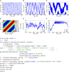
An example showing many of the features of Brian in action. The neuron model in this code follows a stochastic differential equation dV/dT=−(V−El)/τ+σξ(t)/τ, d_Vt_/d_t_ = −(Vt − Vt0)/τ_t_. Here all the undefined symbols are constants except for ≈(t) which corresponds to the term
xi
in the code, and represents a white noise term (〈ξ(t)ξ(t′)〉=δ(t−t′)). The rest of the neuron model is defined by a custom reset function
adaptive_threshold_reset
which increases the value of Vt by a constant each time a neuron spikes (but never takes it above a fixed ceiling), and a custom threshold function
lambda V,Vt:V>=Vt
which defines the condition for a spike. The arguments to the custom reset function are a
NeuronGroup
object
P
(a population of neurons), and an array
spikes
containing the indices of the neurons in
P
that have spiked. Together these two custom functions define an adaptive threshold model. The option to specify custom functions makes Brian's reset and threshold mechanism very flexible. The code also shows synaptic delays, and setting the synaptic weights with a custom function of (i, j),
w*cos(2.*pi*(i-j)*1./100))
. The output of the code shown is the raster plot in (B), with the value
w=.5*mV
. (A) shows
w=.1*mV
and (C) shows
w=.65*mV
. (D) shows the synaptic weight matrix for the
w=.65*mV
case. (E) and (F) show the values of
V
(solid blue) and
Vt
(dashed green) for the neuron with index 50 for the raster plots immediately above them ((B) and (C)) with
w=.5*mV
and
w=.65*mV
respectively.
Figure 3
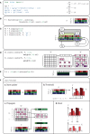
The code from Figure 1 expanded to show how Brian works internally. In (A), the equations for the model are defined. In (B), a group of 4000 neurons is created with these equations. In (C), the logical structure of the network is defined, partitioning the 4000 neurons into excitatory and inhibitory subgroups with corresponding connections to the whole group. In (D), the weight matrices for the excitatory and inhibitory connections are defined. In (E), the membrane potential is initialised uniformly randomly between reset and threshold values. In (F), the simulation is running, consisting of repeated applications of four operations each time step; (a) shows the update of the state matrix; (b) shows the thresholding operation; (c) shows the propagation of spikes; and (d) shows the reset operation.
Figure 4
Computation time for the CUBA network using Brian, C and Matlab. This version of the CUBA network uses a fixed 80 synapses per neuron, and a varying number of neurons N. The figure on the left shows the absolute time on the test machine. The figure on the right shows the time compared to the C code. Theoretically, we would expect O(N) computation time (see Performance of Vectorised Simulations).
Figure 5
Computation time for the CUBA network if all synapses are removed. This largely demonstrates the performance for the state update step, which in this case is a matrix multiplication.
Figure 6
Computation time for the CUBA network with on average p = 500 synapes per neuron and N = 4000 at different firing rates. The parameter we, the excitatory weight, was varied between 1.62 and 4.8 mV which had the effect of varying the firing rate between about 5 Hz and about 25 Hz. This shows how performance scales with the number of spikes. Here the firing rates as well as the times are averaged over the seven fastest trials, as firing rates vary from trial to trial. Note that times due to spiking depend on both the firing rate and the number of synapses per neuron.
Similar articles
- The brian simulator.
Goodman DF, Brette R. Goodman DF, et al. Front Neurosci. 2009 Sep 15;3(2):192-7. doi: 10.3389/neuro.01.026.2009. eCollection 2009 Sep. Front Neurosci. 2009. PMID: 20011141 Free PMC article. - ANNarchy: a code generation approach to neural simulations on parallel hardware.
Vitay J, Dinkelbach HÜ, Hamker FH. Vitay J, et al. Front Neuroinform. 2015 Jul 31;9:19. doi: 10.3389/fninf.2015.00019. eCollection 2015. Front Neuroinform. 2015. PMID: 26283957 Free PMC article. - Brian2CUDA: Flexible and Efficient Simulation of Spiking Neural Network Models on GPUs.
Alevi D, Stimberg M, Sprekeler H, Obermayer K, Augustin M. Alevi D, et al. Front Neuroinform. 2022 Oct 31;16:883700. doi: 10.3389/fninf.2022.883700. eCollection 2022. Front Neuroinform. 2022. PMID: 36387586 Free PMC article. - Code Generation in Computational Neuroscience: A Review of Tools and Techniques.
Blundell I, Brette R, Cleland TA, Close TG, Coca D, Davison AP, Diaz-Pier S, Fernandez Musoles C, Gleeson P, Goodman DFM, Hines M, Hopkins MW, Kumbhar P, Lester DR, Marin B, Morrison A, Müller E, Nowotny T, Peyser A, Plotnikov D, Richmond P, Rowley A, Rumpe B, Stimberg M, Stokes AB, Tomkins A, Trensch G, Woodman M, Eppler JM. Blundell I, et al. Front Neuroinform. 2018 Nov 5;12:68. doi: 10.3389/fninf.2018.00068. eCollection 2018. Front Neuroinform. 2018. PMID: 30455637 Free PMC article. Review. - Simulator for neural networks and action potentials.
Baxter DA, Byrne JH. Baxter DA, et al. Methods Mol Biol. 2007;401:127-54. doi: 10.1007/978-1-59745-520-6_8. Methods Mol Biol. 2007. PMID: 18368364 Review.
Cited by
- Robustness of spiking Deep Belief Networks to noise and reduced bit precision of neuro-inspired hardware platforms.
Stromatias E, Neil D, Pfeiffer M, Galluppi F, Furber SB, Liu SC. Stromatias E, et al. Front Neurosci. 2015 Jul 9;9:222. doi: 10.3389/fnins.2015.00222. eCollection 2015. Front Neurosci. 2015. PMID: 26217169 Free PMC article. - A Diffusive Homeostatic Signal Maintains Neural Heterogeneity and Responsiveness in Cortical Networks.
Sweeney Y, Hellgren Kotaleski J, Hennig MH. Sweeney Y, et al. PLoS Comput Biol. 2015 Jul 9;11(7):e1004389. doi: 10.1371/journal.pcbi.1004389. eCollection 2015 Jul. PLoS Comput Biol. 2015. PMID: 26158556 Free PMC article. - EvtSNN: Event-driven SNN simulator optimized by population and pre-filtering.
Mo L, Tao Z. Mo L, et al. Front Neurosci. 2022 Sep 29;16:944262. doi: 10.3389/fnins.2022.944262. eCollection 2022. Front Neurosci. 2022. PMID: 36248639 Free PMC article. - A circuit motif in the zebrafish hindbrain for a two alternative behavioral choice to turn left or right.
Koyama M, Minale F, Shum J, Nishimura N, Schaffer CB, Fetcho JR. Koyama M, et al. Elife. 2016 Aug 9;5:e16808. doi: 10.7554/eLife.16808. Elife. 2016. PMID: 27502742 Free PMC article. - A neuromorphic spiking neural network detects epileptic high frequency oscillations in the scalp EEG.
Burelo K, Ramantani G, Indiveri G, Sarnthein J. Burelo K, et al. Sci Rep. 2022 Feb 2;12(1):1798. doi: 10.1038/s41598-022-05883-8. Sci Rep. 2022. PMID: 35110665 Free PMC article.
References
- Bower J. M., Beeman D. (1998). The Book of GENESIS: Exploring Realistic Neural Models with the GEneral NEural Simulation System, 2nd edn., Springer-Verlag, New York
- Brette R., Rudolph M., Carnevale T., Hines M., Beeman D., Bower J. M., Diesmann M., Morrison A., Goodman P. H., Harris F. C., Zirpe M., Natschläger T., Pecevski D., Ermentrout B., Djurfeldt M., Lansner A., Rochel O., Vieville T., Muller E., Davison A. P., Boustani S. E., Destexhe A. (2007). Simulation of networks of spiking neurons: a review of tools and strategies. J. Comput. Neurosci. 23, 349–39810.1007/s10827-007-0038-6 - DOI - PMC - PubMed
- Cannon R., Gewaltig M.-O., Gleeson P., Bhalla U., Cornelis H., Hines M., Howell F., Muller E., Stiles J., Wils S., Schutter E. D. (2007). Interoperability of neuroscience modeling software: current status and future directions. Neuroinformatics 5, 127–13810.1007/s12021-007-0004-5 - DOI - PMC - PubMed
- Carnevale N. T., Hines M. L. (2006). The NEURON Book. Cambridge University Press, Cambridge, UK
- Cummins G., Adams R., Newell T. (2008). Scientific computation through a GPU. In Proceedings of the Southeastcon 2008, an IEEE conference, Huntsville, AL, pp. 244–246 http://ieeexplore.ieee.org/xpl/freeabs_all.jsp?arnumber=4494293
LinkOut - more resources
Full Text Sources
Other Literature Sources


