arviz.plot_forest — ArviZ 0.14.0 documentation (original) (raw)
arviz.plot_forest(data, kind='forestplot', model_names=None, var_names=None, filter_vars=None, transform=None, coords=None, combined=False, combine_dims=None, hdi_prob=None, rope=None, quartiles=True, ess=False, r_hat=False, colors='cycle', textsize=None, linewidth=None, markersize=None, legend=True, labeller=None, ridgeplot_alpha=None, ridgeplot_overlap=2, ridgeplot_kind='auto', ridgeplot_truncate=True, ridgeplot_quantiles=None, figsize=None, ax=None, backend=None, backend_config=None, backend_kwargs=None, show=None)[source]#
Forest plot to compare HDI intervals from a number of distributions.
Generates a forest plot of 100*(hdi_prob)% HDI intervals from a trace or list of traces.
Parameters
data: obj or list[obj]
Any object that can be converted to an arviz.InferenceData object Refer to documentation of arviz.convert_to_dataset() for details.
kind: str
Choose kind of plot for main axis. Supports “forestplot” or “ridgeplot”.
model_names: list[str], optional
List with names for the models in the list of data. Useful when plotting more that one dataset.
var_names: list[str], optional
List of variables to plot (defaults to None, which results in all variables plotted) Prefix the variables by ~ when you want to exclude them from the plot.
combine_dimsset_like of str, optional
List of dimensions to reduce. Defaults to reducing only the “chain” and “draw” dimensions. See the this section for usage examples.
filter_vars: {None, “like”, “regex”}, optional, default=None
If None(default), interpret var_names as the real variables names. If “like”, interpret var_names as substrings of the real variables names. If “regex”, interpret var_names as regular expressions on the real variables names. A la pandas.filter.
transform: callable
Function to transform data (defaults to None i.e.the identity function)
coords: dict, optional
Coordinates of var_names to be plotted. Passed to xarray.Dataset.sel().
combined: bool
Flag for combining multiple chains into a single chain. If False(default), chains will be plotted separately.
hdi_prob: float, optional
Plots highest posterior density interval for chosen percentage of density. Defaults to 0.94.
rope: tuple or dictionary of tuples
Lower and upper values of the Region Of Practical Equivalence. If a list with one interval only is provided, the ROPE will be displayed across the y-axis. If more than one interval is provided the length of the list should match the number of variables.
quartiles: bool, optional
Flag for plotting the interquartile range, in addition to the hdi_prob intervals. Defaults to True.
r_hat: bool, optional
Flag for plotting Split R-hat statistics. Requires 2 or more chains. Defaults to False
ess: bool, optional
Flag for plotting the effective sample size. Defaults to False.
colors: list or string, optional
list with valid matplotlib colors, one color per model. Alternative a string can be passed. If the string is cycle, it will automatically chose a color per model from the matplotlibs cycle. If a single color is passed, eg ‘k’, ‘C2’, ‘red’ this color will be used for all models. Defaults to ‘cycle’.
textsize: float
Text size scaling factor for labels, titles and lines. If None it will be autoscaled based on figsize.
linewidth: int
Line width throughout. If None it will be autoscaled based on figsize.
markersize: int
Markersize throughout. If None it will be autoscaled based on figsize.
legendbool, optional
Show a legend with the color encoded model information. Defaults to True, if there are multiple models.
labellerlabeller instance, optional
Class providing the method make_model_label to generate the labels in the plot. Read the Label guide for more details and usage examples.
ridgeplot_alpha: float
Transparency for ridgeplot fill. If 0, border is colored by model, otherwise a black outline is used.
ridgeplot_overlap: float
Overlap height for ridgeplots.
ridgeplot_kind: string
By default (“auto”) continuous variables are plotted using KDEs and discrete ones using histograms. To override this use “hist” to plot histograms and “density” for KDEs.
ridgeplot_truncate: bool
Whether to truncate densities according to the value of hdi_prob. Defaults to True.
ridgeplot_quantiles: list
Quantiles in ascending order used to segment the KDE. Use [.25, .5, .75] for quartiles. Defaults to None.
figsize: tuple
Figure size. If None, it will be defined automatically.
ax: axes, optional
matplotlib.axes.Axes or bokeh.plotting.Figure.
backend: str, optional
Select plotting backend {“matplotlib”,”bokeh”}. Defaults to “matplotlib”.
backend_config: dict, optional
Currently specifies the bounds to use for bokeh axes. Defaults to value set in rcParams.
backend_kwargs: bool, optional
These are kwargs specific to the backend being used, passed tomatplotlib.pyplot.subplots() or bokeh.plotting.figure(). For additional documentation check the plotting method of the backend.
show: bool, optional
Call backend show function.
Returns
gridspec: matplotlib GridSpec or bokeh figures
See also
Plot Posterior densities in the style of John K. Kruschke’s book.
Generate KDE plots for continuous variables and histograms for discrete ones.
Examples
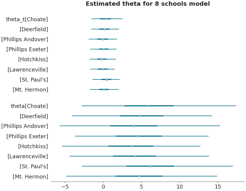
Forestplot
import arviz as az non_centered_data = az.load_arviz_data('non_centered_eight') axes = az.plot_forest(non_centered_data, kind='forestplot', var_names=["^the"], filter_vars="regex", combined=True, figsize=(9, 7)) axes[0].set_title('Estimated theta for 8 schools model')
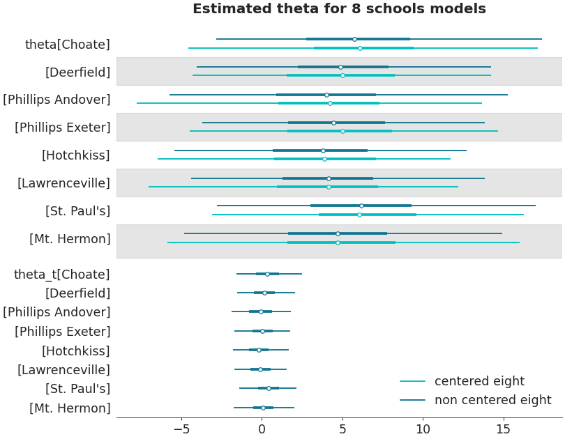
Forestplot with multiple datasets
centered_data = az.load_arviz_data('centered_eight') axes = az.plot_forest([non_centered_data, centered_data], model_names = ["non centered eight", "centered eight"], kind='forestplot', var_names=["^the"], filter_vars="regex", combined=True, figsize=(9, 7)) axes[0].set_title('Estimated theta for 8 schools models')
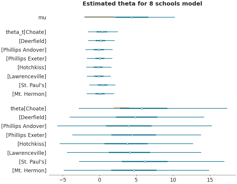
Forestplot with ropes
rope = {'theta': [{'school': 'Choate', 'rope': (2, 4)}], 'mu': [{'rope': (-2, 2)}]} axes = az.plot_forest(non_centered_data, rope=rope, var_names='~tau', combined=True, figsize=(9, 7)) axes[0].set_title('Estimated theta for 8 schools model')
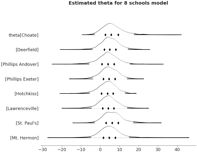
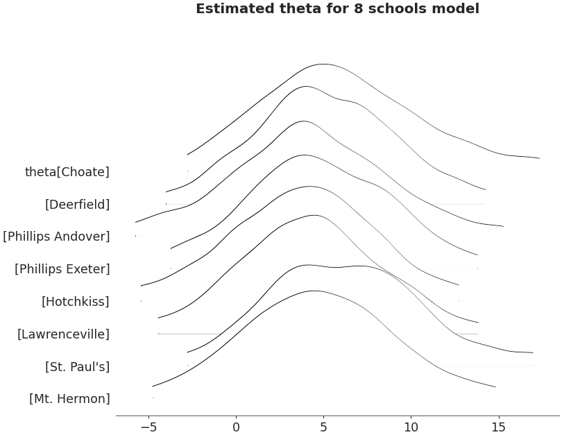
Ridgeplot
axes = az.plot_forest(non_centered_data, kind='ridgeplot', var_names=['theta'], combined=True, ridgeplot_overlap=3, colors='white', figsize=(9, 7)) axes[0].set_title('Estimated theta for 8 schools model')
Ridgeplot non-truncated and with quantiles
axes = az.plot_forest(non_centered_data, kind='ridgeplot', var_names=['theta'], combined=True, ridgeplot_truncate=False, ridgeplot_quantiles=[.25, .5, .75], ridgeplot_overlap=0.7, colors='white', figsize=(9, 7)) axes[0].set_title('Estimated theta for 8 schools model')