Constraint Propagation in AI (original) (raw)
Last Updated : 27 May, 2026
Constraint Propagation is a technique used in Artificial Intelligence to solve Constraint Satisfaction Problems (CSPs). It works by reducing the possible values of variables using given constraints, which helps narrow the search space and improve problem-solving efficiency.
- Helps eliminate invalid values from variable domains
- Reduces the complexity of CSPs before search begins
- Commonly used in scheduling, planning, and resource allocation
Key Concepts
- **Variables: In constraint satisfaction problems (CSPs), variables are the elements that need to be assigned specific values. These variables represent the unknowns in a problem.
- **Domains: A domain is the set of all possible values that can be assigned to a variable. Constraint propagation reduces these domains by removing values that violate constraints.
- **Constraints: Constraints are rules that define valid relationships between variables and restrict unacceptable value combinations. They help ensure that the final solution satisfies all problem conditions.
Working
Constraint propagation works by reducing the possible values of variables using the given constraints. This process continues until no more values can be removed from the domains of the variables.
Let’s consider two variables X and Y, each having the domain \{1,2,3\} with the constraint X \ne Y.
**Step 1: Initialization
Initially, both variables can take any value from their domains.
X = \{1,2,3\}, Y = \{1,2,3\}
**Step 2: Apply Constraints
Suppose X = 1. Since X \ne Y, the value 1 is removed from the domain of Y.
Y = \{2,3\}
**Step 3: Further Propagation
Now, ifY = 2****,** then X cannot be 2 due to the same constraint.
X = \{1,3\}
Step 4: Iteration
The process continues by repeatedly applying constraints and reducing domains until no more values can be eliminated.
Step 5: Stable State
When no further reductions are possible, the domains reach a stable state, making it easier to identify valid solutions efficiently.
Algorithms Used
- **Arc Consistency (AC-3): Ensures that for every value of one variable, there is at least one compatible value in the connected variable that satisfies the constraint. It is commonly used to reduce domains before solving the CSP.
- **Path Consistency: Extends arc consistency by considering relationships among three variables. It checks whether values between two variables remain consistent when a third variable is involved, helping further reduce the search space.
- **k-Consistency: A generalized form of consistency that works with k variables. It ensures that if values are assigned to k-1 variables, there exists a valid value for the k^{th} variable that satisfies all constraints.
- **Singleton Consistency: Temporarily assigns a single value to a variable and checks whether the CSP remains consistent. It helps detect invalid assignments early and is useful in puzzle-solving problems.
- **Generalized Arc Consistency (GAC): An advanced form of arc consistency used for constraints involving multiple variables. It ensures that every value in a variable’s domain satisfies the constraint with compatible values in the domains of other related variables.
Implementation
Here, we will be implementing a basic constraint satisfaction problem (CSP) solver using arc consistency using Python.
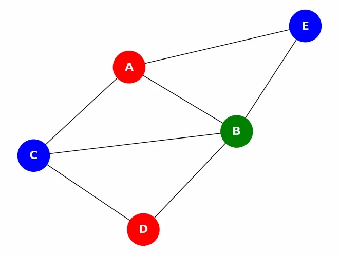
Let's say we have a map with five regions (A, B, C, D, E) and we need to assign one of three colors (Red, Green, Blue) to each region. The constraint is that no two adjacent regions can have the same color.
Step 1: Importing Required Libraries
Here we will be using Matplotlib and Networkx libraries for this implementation.
Python `
import matplotlib.pyplot as plt import networkx as nx
`
Step 2: Defining the CSP Class
We define a CSP class to store variables, domains, neighbors, and constraints, providing a structured framework to model and solve the constraint satisfaction problem.
Python `
class CSP: def init(self, variables, domains, neighbors, constraints): self.variables = variables self.domains = domains self.neighbors = neighbors self.constraints = constraints
`
Step 3: Consistency Checking Method
The consistency check method verifies whether the current variable assignment satisfies all constraints and returns False if any constraint is violated.
Python `
def is_consistent(self, var, assignment): """Check if an assignment is consistent by checking all constraints.""" for neighbor in self.neighbors[var]: if neighbor in assignment and not self.constraints(var, assignment[var], neighbor, assignment[neighbor]): return False return True
`
Step 4: AC-3 Algorithm Method
Implementing the AC-3 algorithm to enforce arc consistency by reducing variable domains and removing values that have no valid support in neighboring variables.
Python `
def ac3(self): """AC-3 algorithm for constraint propagation.""" queue = [(xi, xj) for xi in self.variables for xj in self.neighbors[xi]] while queue: (xi, xj) = queue.pop(0) if self.revise(xi, xj): if len(self.domains[xi]) == 0: return False for xk in self.neighbors[xi]: if xk != xj: queue.append((xk, xi)) return True
`
Step 5: Revising Method
The revise method refines the domain of a variable by removing values that do not meet the constraints with its neighbors. It reduces the search space by eliminating inconsistent assignments which simplifies the problem.
Python `
def revise(self, xi, xj): """Revise the domain of xi to satisfy the constraint between xi and xj.""" revised = False for x in set(self.domains[xi]): if not any(self.constraints(xi, x, xj, y) for y in self.domains[xj]): self.domains[xi].remove(x) revised = True return revised
`
Step 6: Backtracking Search Method
Backtracking tries different variable assignments and, on conflicts, revisits earlier choices until a valid solution is found or all possibilities are exhausted.
Python `
def backtracking_search(self, assignment={}): """Backtracking search to find a solution.""" if len(assignment) == len(self.variables): return assignment
var = self.select_unassigned_variable(assignment)

for value in self.domains[var]:
    new_assignment = assignment.copy()
    new_assignment[var] = value
    if self.is_consistent(var, new_assignment):
        result = self.backtracking_search(new_assignment)
        if result:
            return result

return None
`
Step 7: Selecting Unassigned Variable Method
This method selects an unassigned variable, often choosing the one with the fewest remaining values to reduce the search space and improve efficiency.
Python `
def select_unassigned_variable(self, assignment): """Select an unassigned variable (simple heuristic).""" for var in self.variables: if var not in assignment: return var return None
`
Step 8: Constraint Function
The constraint function ensures that adjacent regions do not share the same color by validating each assignment against the map coloring rules.
Python `
def constraint(var1, val1, var2, val2): """Constraint function: no two adjacent regions can have the same color.""" return val1 != val2
`
Step 9: Visualizing Function
The visualization function plots the map using Network and Matplotlib. It visually shows the result by coloring the regions according to the solution found, making the solution easier to interpret.
Python `
def visualize_solution(solution, neighbors): """Visualize the solution using matplotlib and networkx.""" G = nx.Graph() for var in solution: G.add_node(var, color=solution[var]) for var, neighs in neighbors.items(): for neigh in neighs: G.add_edge(var, neigh)
colors = [G.nodes[node]['color'] for node in G.nodes]
pos = nx.spring_layout(G)
nx.draw(G, pos, with_labels=True, node_color=colors, node_size=2000,
        font_size=16, font_color='white', font_weight='bold')
plt.show()
`
Step 10: Defining Variables, Domains and Neighbors
We define variables (regions), domains (colors), and neighbors (adjacent regions) to structure the CSP and establish relationships for constraint checking.
Python `
variables = ['A', 'B', 'C', 'D', "E"] domains = { 'A': ['Red', 'Green', 'Blue'], 'B': ['Red', 'Green', 'Blue'], 'C': ['Red', 'Green', 'Blue'], 'D': ['Red', 'Green', 'Blue'], 'E': ['Red', 'Green', 'Blue'] }
neighbors = { 'A': ['B', 'C'], 'B': ['A', 'C', 'D'], 'C': ['A', 'B', 'D'], 'D': ['B', 'C'], 'E': ['A', 'B'] }
`
Step 11: Creating CSP Instance and Applying AC-3 Algorithm
We create an instance of the CSP class and apply the AC-3 algorithm to propagate constraints and reduce the domains followed by backtracking search to find a valid solution.
Python `
csp = CSP(variables, domains, neighbors, constraint)
if csp.ac3():
solution = csp.backtracking_search()

if solution:

    print("Solution found:")

    for var in variables:
        print(f"{var}: {solution[var]}")

    visualize_solution(solution, neighbors)

else:
    print("No solution found")
else: print("No solution found")
`
**Output:
Solution found:
A: Red
B: Green
C: Blue
D: Red
E: Blue
Output
Applications
- **Scheduling: Assigns tasks to time slots while avoiding conflicts and respecting constraints like availability and dependencies.
- **Planning: Reduces possible actions at each step to build valid sequences that achieve a goal efficiently.
- **Resource Allocation: Assigns limited resources to tasks while satisfying constraints such as capacity and priority rules.
- **Cryptographic Protocol Design: Helps eliminate invalid configurations of keys and protocols by enforcing security constraints, ensuring only secure and valid setups are considered.
- **Vehicle Routing Problems (VRP): Improves route planning by enforcing constraints like delivery time windows, vehicle capacity, and distance limits, helping in finding efficient and feasible delivery routes.
Advantages
- Improves efficiency by reducing the search space early through removal of invalid values, making solving faster.
- Enhances scalability by breaking complex problems into smaller, manageable subproblems.
- Offers flexibility across domains like scheduling, planning, and resource allocation with different constraint types.
- Reduces computation by pruning large parts of the search space at early stages.
- Maintains consistency by ensuring partial solutions satisfy constraints, reducing backtracking.
Limitations
- Higher computational cost is required for strong consistency methods like arc or k-consistency, especially in large problems.
- May not fully reduce variable domains, leaving multiple possibilities that still require backtracking or other search methods.
- Adds overhead in simple problems where constraints are weak or not highly interconnected.
- Has limited effectiveness for complex or dynamic problems that need more advanced or hybrid solving techniques.