Empirical Distribution Function (EDF) (original) (raw)

Last Updated : 23 Jul, 2025

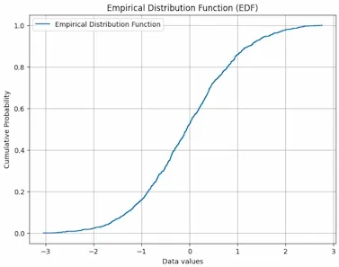
The Empirical Distribution Function is a method used to estimate the cumulative distribution function (CDF) based on a sample. It provides an estimate of the proportion of data points in the sample that are less than or equal to a particular value. The theoretical CDF is based on assumptions about the population distribution whereas the EDF is derived directly from observed data which makes it flexible and widely applicable to real-world datasets. EDF is defined as:

F_n(x) = \frac{\text{Number of points} \leq x}{n}

Where:

F_n(x) is the empirical distribution function at the value x,
n is the total number of data points in the sample,
The numerator is the count of data points that are less than or equal to x.

In simplified terms the EDF at any given point x represents the fraction of data points that are smaller than or equal to that value.

Key Characteristics

**Step Function: It is a step function, where each step occurs at a data point and the height of the step represents the cumulative probability up to that data point.
**Non-decreasing: It is always a non-decreasing function. As we move along the data points in ascending order, the cumulative probability either increases or stays the same.
**Right-continuous: The function takes the value corresponding to the right-hand side of the step.

Step-by-Step Process for Calculating the EDF

**1. Sort the Data: Sort the values in increasing order.

**2. Compute the EDF: For each sorted value (x_i), compute the cumulative probability:

F_n(x_i) = \frac{i}{n}

Where i is the rank of the data point x_i in the sorted list, i.e., the number of values less than or equal to x_i.

**3. Graph the EDF: The EDF can be plotted as a step function, with the sorted data values on the x-axis and the cumulative probability on the y-axis.

Example-graph-to-shoe-EDF-plotting

Example to show EDF Plotting

Example

**1. Data Sample: Suppose we have a dataset of 5 values [2,9,12,7,5].

**2. Sort the Data: Sort the data in ascending order [2,5,7,9,12].

**3. Compute the EDF: Lets calculate the EDF for each sorted value,

For x=2, 1 value is less than or equal to 2 so,

F_n(2) = \frac{1}{5} = 0.2

For x=5, 2 values are less than or equal to 5 so,

F_n(5) = \frac{2}{5} = 0.4

For x=7, 3 value are less than or equal to 7 so,

F_n(7) = \frac{3}{5} = 0.6

For x=9, 4 value are less than or equal to 9 so,

F_n(9) = \frac{4}{5} = 0.28

For x=12, 5 value are less than or equal to 12 so,

F_n(12) = \frac{5}{5} = 1.0

**4. Plot the EDF:

EDF_example_RESULT

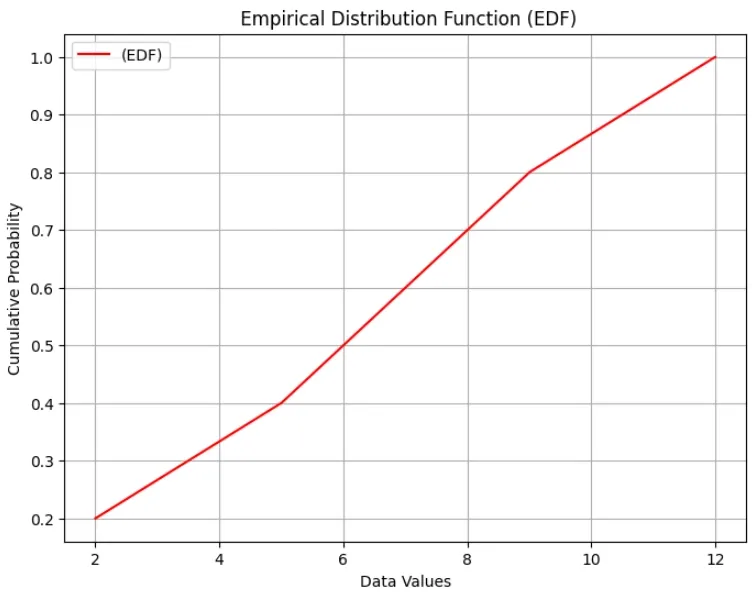
Representation of the Result of EDF on given dataset

Applications of the EDF

**Goodness-of-Fit Tests: It is useful in tests like the Kolmogorov-Smirnov test, which compares the EDF of a sample with a theoretical distribution (e.g., normal distribution) to see how well the data matches the assumed model.
**Data Comparison: We can compare two datasets by plotting their EDFs on the same graph. This helps us visually check how similar or different their distributions are, useful for comparing different groups or testing hypotheses.

comparison-of-EDF

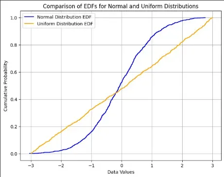
Example to show EDF Comparison

**Visualizing Data Distribution: It provides a simple way to visualize how data is distributed. By looking at the plot we can see how the data spreads, where it's concentrated and if there are any outliers.
**Non-Parametric Statistics: It is used for analyzing data that doesn't follow standard distributions, like skewed or uniform data.

Limitations of EDF

**Sensitive to Sample Size: The EDF becomes more accurate with larger datasets; small samples may not represent the true distribution well.
**Step Function: It is may miss subtle data patterns especially in highly variable data.
**Limited Tail Information: It doesn’t provide detailed insights into the distribution's tails (extreme values).
**Struggles with Outliers: It may not accurately represent datasets with significant outliers.