Markov chain Monte Carlo (MCMC) (original) (raw)
Last Updated : 24 Oct, 2025
Markov Chain Monte Carlo (MCMC) is a method to sample from a probability distribution when direct sampling is hard. It builds a Markov chain that moves step by step, visiting points that follow the target distribution. The more steps taken, the closer the samples get to the true distribution. It is composed of two components- Monte Carlo and Markov Chain. Lets understand them separately.
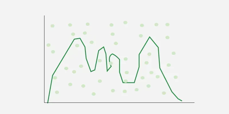
Figure 1- Monte Carlo method to estimate area under curve
**Monte Carlo Sampling
**Monte Carlo Sampling is a technique for sampling a probability distribution and then using those samples to approximate desired quantity, i.e it uses randomness to estimate some deterministic quantity of interest.
Example: To find the area under the curve in figure-1, instead of complex integration we use the Monte Carlo method. We randomly place green dots inside the rectangle to improve accuracy, then find the ratio of dots under the curve to total dots. Multiplying this ratio by the rectangle’s area gives an estimate of the area under the curve.
Lets understand Monte Carlo method Mathematically, suppose we have Expectation (s) to estimate, this might be a highly complex integral or challenging to be estimated whereas using the Monte Carlo method we get the estimated values by taking the average of multiple random samples. Original expectations can be calculated by
s = \int p(x) f(x) \, dx = \mathbb{E}_{p}[f(x)]
whereas the approximated expectation that would be generated by stimulating large samples of f(x) can be achieved by:
\hat{s}_n = \frac{1}{n} \sum_{i=1}^{n} f(x^{(i)})
Computing the average over a large number of samples could reduce the standard error and give us a fairly accurate approximation.
**Markov Chains
**Markov Chains can be understood as a process of moving step-by-step through states where the choice of the next state depends only on the current state and the probability distribution of possible next states. Let's have a look at Markov Property,
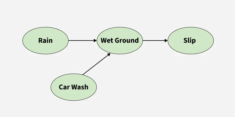
Entities in the oval shapes are different states
Lets consider a system of 4 states as shown, 'Rain' or 'Car Wash" causing the 'Wet Ground' which is the followed by 'Slip'. Markov property simply makes an assumption that the probability of jumping from one state to the next state depends only on the current state not on the sequence of previous states which lead to this state. Mathematically it is:
P(X_{n+1} = k \mid X_n = k_n, X_{n-1} = k_{n-1}, \ldots, X_1 = k_1) = P(X_{n+1} = k \mid X_n = k_n)
It is quite evident from the mathematical equation that the Markov Property assumption could potentially save computational energy and time. If a process exhibits Markov Property then it is known as Markov Chain.
Markov Chain Monte Carlo
Markov Chain Monte Carlo is widely used in Bayesian inference to approximate posterior distributions that are often hard to compute exactly. Lets understand the challenge of Bayesian Inference. Bayes theorem lets us update our beliefs about unknown parameters by combining prior knowledge with observed data. Mathematically the posterior distribution is proportional to the likelihood multiplied by the prior:
P(\theta \mid \text{data}) \propto P(\text{data} \mid \theta) \times P(\theta)
But to get the exact posterior we must divide by the marginal likelihood or evidence:
P(\text{data}) = \int P(\text{data} \mid \theta) \, P(\theta) \, d\theta
This marginal probability acts as a normalisation constant to ensure the posterior integrates to one. But calculating this integral is often computationally expensive or impossible for complex models. To avoid directly calculating the normalisation constant, MCMC constructs a Markov chain whose long-run behaviour matches the target posterior distribution. The basic idea is:
- Start with any initial state in the parameter space.
- Generate a sequence of states (samples) by moving step-by-step, guided by transition rules.
- These rules ensure the chain spends more time in areas where the posterior probability is higher.
- Over the time, these sampled states converges to the true posterior.
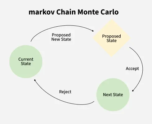
Figure 3- Markov Chain Monte Carlo overview
Ensuring Convergence
Markov Chain Monte Carlo enforces the detailed balance condition so as to guarantee that the chain settles into the target distribution. This condition requires that the flow of probability from one state A to another B equals the flow from B back to A:
\pi(A) \cdot T(A \rightarrow B) = \pi(B) \cdot T(B \rightarrow A)
Here π is the target distribution (posterior) and T (x → y) is the probability of moving from state x to state y.
**How Markov Chain Monte Carlo Works
- **Start with a point: Pick an initial value or state from the space.
- **Propose a move: Generate a candidate for the next state based on proposal rule.
- **Evaluate the move: Calculate how likely this new state is compared to the current state, based on the target distribution.
- **Decide to accept or reject: If the new state is more likely then it is accepted but if less likely then accept it with probability proportional to how less likely it is.
- **Repeat steps 2-4: Continue proposing and accepting/rejecting new states for several times and over time the collected states (samples) will represent the target distribution.
- **Burn-in period: Discard initial samples until the chain "forgets" its starting point and reaches steady behavior.
- **Collect samples: Use the remaining samples to estimate properties of the target distributions.
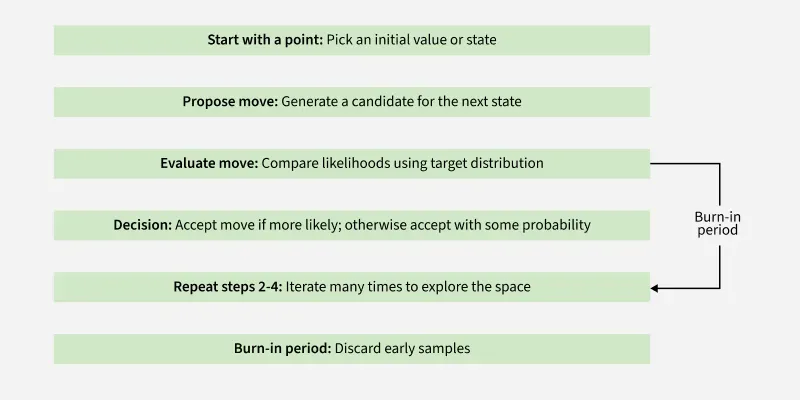
Figure 4- Markov Chain Monte Carlo Working Sample
Metropolis - Hasting Algorithm
Suppose we are sampling from distribution p(x) = f(x) / Z where Z is the normalization constant. Our objective is to sample from p(x) in such a way that involves making use of numerator alone and avoids having to estimate denominator. Looking at the proposal probability(g) we will start.
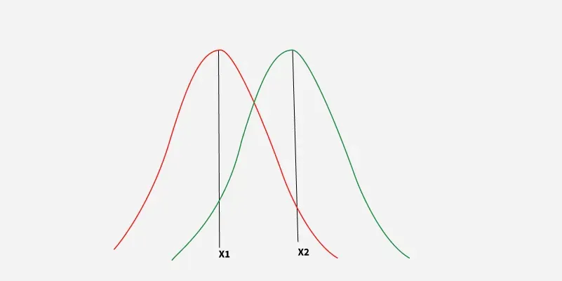
Figure 5- Proposal Distribution
**Step-by-step process:
1.**Start at an initial state X 1 : We choose a starting point.
2.**Propose a new state X 2 : Generate a candidate state from a proposal distribution g(X_2 \mid X_1) like a normal distribution centered at X1.
3.**Evaluate the move: Compute the unnormalized density ratio:
R_f = \frac{f(X_2)}{f(X_1)}
And the proposal distribution ratio:
R_g = \frac{g(X_1 \mid X_2)}{g(X_2 \mid X_1)}
4. **Decide to accept or reject: Calculate the acceptance probability:
A(X_1 \rightarrow X_2) = \min\left(1, R_f \cdot R_g\right)
Accept X2 with this probability otherwise remain at X1.
5.**Burn-in period: Discard initial samples until the chain reaches a stationary state.
6. **Collect samples: Use the remaining samples to estimate properties of the target distribution.
**Detailed Balance Condition:
p(X_1) \cdot g(X_1 \mid X_2) \cdot A(X_1 \rightarrow X_2) = p(X_2) \cdot g(X_2 \mid X_1) \cdot A(X_2 \rightarrow X_1)
Replace **p(x) with unnormalised target density **f(x)/Z (since Z cancels out):
f(X_1) \cdot g(X_1 \mid X_2) \cdot A(X_1 \rightarrow X_2) = f(X_2) \cdot g(X_2 \mid X_1) \cdot A(X_2 \rightarrow X_1)
Rearranging:
\frac{A(X_2 \rightarrow X_1)}{A(X_1 \rightarrow X_2)} = \frac{f(X_1)}{f(X_2)} \cdot \frac{g(X_1 \mid X_2)}{g(X_2 \mid X_1)}
Using shorthand:
R_f = \frac{f(X_2)}{f(X_1)}, \quad R_g = \frac{g(X_2 \mid X_1)}{g(X_1 \mid X_2)} \Rightarrow \frac{A(X_1 \rightarrow X_2)}{A(X_2 \rightarrow X_1)} = R_f \cdot R_g
Assuming:
A(X_2 \rightarrow X_1) = 1(if the reverse move is always accepted)
Final Acceptance Rule:
A(X_1 \rightarrow X_2) = \min\left(1, R_f \cdot R_g \right)
And if the proposal distribution is symmetric(like Normal), then:
g(X_2 \mid X_1) = g(X_1 \mid X_2) \Rightarrow R_g = 1
And the rule simplifies to:
A(X_1 \rightarrow X_2) = \min\left(1, \frac{f(X_2)}{f(X_1)}\right)
Comparison of Markov Chain Monte Carlo with Other Sampling Methods:
| Feature | MCMC | Rejection Sampling | Importance Sampling |
|---|---|---|---|
| Scalability to High Dimensions | High- handles complex, high dimensional spaces | Poor- becomes inefficient as dimensions grow | Poor- performance degrades in high dimensions |
| Adaptability to Posterior Shape | High-Samples according to target shape. | Low | Moderate- sensitive to choice of proposal distribution |
| Flexibility in Model Complexity | High | Limited- not suited for complex models | Moderate |
| Computational Efficiency | Moderate- computationally intensive but accurate | Low- many samples are rejected | Moderate- efficiency depends on proposal |
Applications
- **Bayesian Inference: MCMC approximates complex posterior distributions for parameter estimation and uncertainty quantification when exact solutions are unavailable.
- **Econometrics & Finance: Used for modeling financial time series with stochastic and hierarchical Bayesian models hence improving forecasting and risk analysis.
- **Machine Learning & AI: Applied in training probabilistic graphical models and Bayesian deep learning for uncertainty-aware predictions.
- **Natural Language Processing (NLP): Helps infer latent linguistic structures in topic modeling, parsing and word sense disambiguation.
Advantages
- **Handles Complex Models: Effective for high-dimensional models like Bayesian neural networks and probabilistic graphical models.
- **Supports Bayesian Inference in NLP Tasks: Enables posterior estimation in models with complex likelihoods like LDA or parsing.
- **Full Posterior Distributions: Provides a complete uncertainty picture beyond point estimates like MLE or MAP.
- **Integration with Semi/Unsupervised Learning: Useful for clustering, generative modeling and data augmentation.
Challenges
- **Convergence Issues: Requires careful tuning to ensure the chain reaches the target distribution.
- **Computationally Intensive: Can be slow and costly, especially with high-dimensional data.
- **Long Mixing Times: Slow convergence leads to poor sampling efficiency.