Markov Chain (original) (raw)
Last Updated : 31 Jul, 2025
A Markov chain is a way to describe a system that moves between different situations called "states", where the chain assumes the probability of being in a particular state at the next step depends solely on the current state. This key property of ignoring historical states is called the Markov Property or memorylessness.
Fundamental Properties
1. **Irreducibility: It is possible to reach any state from any other (maybe through several steps).
2. **Periodicity: A state is periodic if returns are only possible at multiples of some step (>1).
- Transience and Recurrence:
- Transient: The system might never return to this state.
- Recurrent: The system is certain to return eventually.
- Absorbing States: Once entered, the process cannot leave i.e. no outgoing transitions.
Visualizing a Markov Chain
Consider a Markov chain with two possible states, A and E. The process can either stay in the same state or transition to the other, each with a particular probability.
**Example: Two-State Markov Process
If in state A:
- Stays in A: probability 0.6
- Moves to E: probability 0.4
If in state E:
- Moves to A: probability 0.7
- Stays in E: probability 0.3
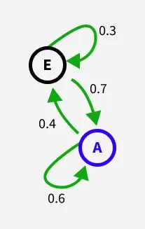
State Transition Diagram
A Markov chain can be illustrated as a directed graph, where:
- Nodes represent the states (A, E)
- Arrows indicate possible transitions
- Numbers on arrows show transition probabilities
Transition Matrix
A Markov chain can be represented by a transition matrix:
| A | E | |
|---|---|---|
| A | 0.6 | 0.4 |
| E | 0.7 | 0.3 |
Each row corresponds to the current state and each column to the future state. The value in each cell is the probability of moving from the row’s state to the column’s state. Each row sums to 1.
- Transition matrix for N states is always N \times N.
- The initial state vector (N \times 1) specifies starting probabilities.
N-Step Transition Matrices
To find probabilities of transitions over multiple steps, raise the transition matrix to the power of N :
P_{\text{n steps}} = \left(P_{\text{1 step}}\right)^n
The entry at position (A, E) in the resulting matrix gives the chance of moving from A to E in N steps.
Types of Markov Chains
**1. Discrete-Time Markov Chains (DTMC):
- State changes occur at specific, countable time steps.
- Most references to "Markov chain" assume discrete time by default.
**2. Continuous-Time Markov Chains (CTMC): State changes can occur at any instant (time is continuous).
Step-by-step Implementation of Markov Chain
Step 1: Import Required Libraries.
- numpy makes it easy to handle numerical data and arrays.
- scipy.linalg contains functions to compute eigenvectors, which are needed to find the stationary distribution. Python `
import numpy as np import scipy.linalg
`
Step 2: Define States and Transition Matrix
**transition_matrix**is a 2x2 array where each row gives the probabilities of moving from one state to another.
- Row 0 (
[0.6, 0.4]) is for state "A": 60% chance to stay in "A", 40% to move to "E". - Row 1 (
[0.7, 0.3]) is for state "E": 70% chance to move to "A", 30% to stay in "E". Python `
states = ["A", "E"] transition_matrix = np.array([[0.6, 0.4], [0.7, 0.3]])
`
Step 3: Simulate a Random Walk on the Markov Chain
n_stepscontrols how many transitions will occur.current_state = 0means we begin at state "A".np.random.choice(, p=...)randomly picks the next state (0 for "A", 1 for "E") based on the transition probabilities from the current state.- This simulates the Markov property: the next state depends only on the current state, not the history. Python `
n_steps = 20 current_state = 0
print(states[current_state], end=" -> ") for _ in range(n_steps - 1): current_state = np.random.choice( [0, 1], p=transition_matrix[current_state]) print(states[current_state], end=" -> ") print("stop")
`
Step 4: Find the Stationary Distribution
- The stationary distribution tells us the long-run probability of being in each state, regardless of where we started.
- We compute the left eigenvectors (with
left=True) of the transition matrix. - The stationary distribution corresponds to the eigenvector associated with eigenvalue 1.
.realensures we're only using the real part (sometimes eigenvectors can have a small imaginary component due to numerical computation).- **
stationary /= stationary.sum():**normalizes the vector so all entries add up to 1 (since probabilities must sum to 1). Python `
eigvals, left_eigvecs = scipy.linalg.eig( transition_matrix, left=True, right=False) stationary = left_eigvecs[:, 0].real stationary /= stationary.sum() print("Stationary distribution:", stationary)
`
Applications of Markov Chain
- **Web Search (PageRank Algorithm): Google’s PageRank uses Markov chains to rank web pages by modeling random web surfing as transitions between pages.
- **Natural Language Processing & Speech Recognition: Markov models, especially Hidden Markov Models (HMMs), are fundamental to speech recognition and text modeling, enabling applications like voice assistants and predictive typing.
- **Finance and Economics: Markov chains model market behavior, such as stock price movements, business cycles (recession/expansion), credit rating transitions and risk predictions.
- **Biology and Genetics: Used to model genetic sequences, protein structures, population dynamics and disease spread, making them essential in bioinformatics and epidemiology.
- **Markov Chain Monte Carlo (MCMC) Methods in Statistics and Simulation: It is the backbone of many modern statistical methods, MCMC uses Markov processes to sample complex probability distributions for Bayesian inference, physics and machine learning
Advantages
- **Simplicity: Markov chains use straightforward mathematical formulations. Once the transition probabilities are set, modeling is simple and easy to interpret.
- **Memorylessness: The Markov property (memorylessness) often matches real-world systems, where the next state depends only on the current state, not the full history.
- **Computational Efficiency: Calculations involving future probabilities, stationary distributions or multi-step transitions can be performed efficiently using matrix algebra.
- **Foundation for Complex Models: Markov chains are the basis for more advanced frameworks like Hidden Markov Models (HMMs) and Markov Decision Processes (MDPs), which are essential in AI, robotics and speech recognition.
Limitations
- **Fixed Transition Probabilities: Standard Markov chains assume transition probabilities don't change over time, which may not reflect real-world dynamics.
- **Discrete States: Classical Markov chains handle finite or countable states and may not be ideal for systems with continuous variables.
- **Limited to Short-term Dependencies: They can't model long-range dependencies or delayed effects efficiently without increasing model complexity like using higher-order chains.
- **State Space Explosion: For systems with many features/states, the number of possible states grows rapidly making computation and interpretation difficult.