Fast Fourier Transform in Image Processing (original) (raw)

Last Updated : 11 Jun, 2026

Fast Fourier Transform (FFT) is a mathematical algorithm that converts an image between the spatial domain and the frequency domain, helping with image filtering, compression and enhancement.

• Spatial domain represents an image using pixel values.
• Frequency domain represents an image using intensity variation patterns.
• Low frequencies correspond to smooth regions and gradual changes.
• High frequencies correspond to edges, fine details and sharp changes.
• Frequency domain shows the contribution of different frequency components in an image.

Implementing Fast Fourier Transform

The Fast Fourier Transform (FFT) processes an image in three main steps

1. **Forward FFT: Converts the image from the spatial domain to the frequency domain, representing it in terms of frequency components.
2. **Frequency Domain Processing: Filters are applied to modify specific frequencies for tasks such as noise removal, image enhancement and sharpening.
3. **Inverse FFT (Frequency to Spatial Domain): Converts the modified frequency data back to the spatial domain to obtain the processed image.

1. Image Transformation using FFT

This technique converts an image from the spatial domain to the frequency domain, allowing us to analyze the frequency components present in the image.

• The image is first converted to grayscale for processing.
• fft2() applies the Fast Fourier Transform to obtain the frequency representation of the image.
• fftshift() moves the low-frequency components to the center of the spectrum for easier visualization.
• The magnitude spectrum is calculated to show the strength of different frequency components. Python `

import numpy as np import cv2 import matplotlib.pyplot as plt import requests from PIL import Image from io import BytesIO

url = "https://encrypted-tbn0.gstatic.com/images?q=tbn:ANd9GcRmKTFI_7r2TKR0sknfK_7GJX8sHItxbf-zh_jOJIBde2-L69K29IAzFLrD&s"

response = requests.get(url) img_data = response.content

img = Image.open(BytesIO(img_data))

img_gray = np.array(img.convert('L'))

f = np.fft.fft2(img_gray) fshift = np.fft.fftshift(f)

magnitude_spectrum = 20 * np.log(np.abs(fshift))

plt.figure(figsize=(12, 6)) plt.subplot(121), plt.imshow(img_gray, cmap='gray'), plt.title('Original Image') plt.subplot(122), plt.imshow(magnitude_spectrum, cmap='gray'), plt.title('Magnitude Spectrum') plt.show()

`

**Output:

Image Transformation

2. Low-Pass Filtering

A Low-Pass Filter (LPF) removes high frequency components from an image while preserving low frequency information. This reduces noise and fine details, producing a smoother or blurred image.

• The image is converted to grayscale and transformed to the frequency domain using FFT.
• A low-pass filter mask is created to keep only the low frequency components near the center of the spectrum.
• High frequency components outside the mask are removed.
• The filtered frequency data is converted back to the spatial domain using the Inverse FFT.
• The resulting image appears smoother with reduced details and noise. Python `

import numpy as np import cv2 import matplotlib.pyplot as plt import requests from PIL import Image from io import BytesIO

url = "https://encrypted-tbn0.gstatic.com/images?q=tbn:ANd9GcRmKTFI_7r2TKR0sknfK_7GJX8sHItxbf-zh_jOJIBde2-L69K29IAzFLrD&s"

response = requests.get(url) img_data = response.content

img = Image.open(BytesIO(img_data))

image = np.array(img.convert('L'))

f = np.fft.fft2(image) fshift = np.fft.fftshift(f)

rows, cols = image.shape crow, ccol = rows // 2, cols // 2 mask = np.zeros((rows, cols), np.uint8) mask[crow-30:crow+30, ccol-30:ccol+30] = 1

fshift_masked = fshift * mask f_ishift = np.fft.ifftshift(fshift_masked) image_filtered = np.fft.ifft2(f_ishift) image_filtered = np.abs(image_filtered)

plt.imshow(image_filtered, cmap='gray') plt.title('Low-Pass Filtered Image') plt.show()

`

**Output:

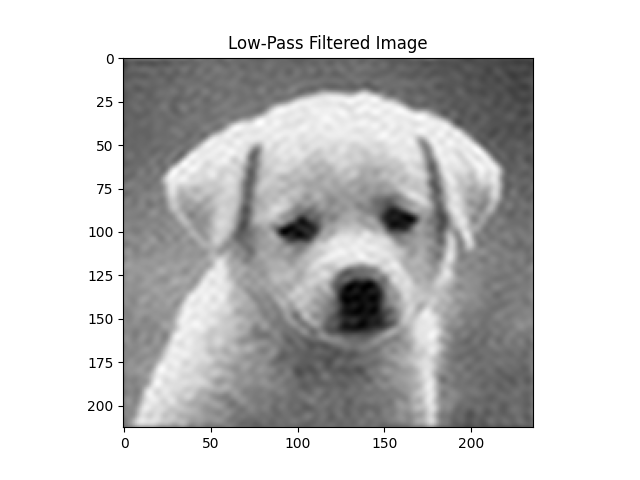
Low-Pass Filtering

3. High-Pass Filtering

A High-Pass Filter (HPF) removes low frequency components and preserves high-frequency components, helping enhance edges and fine details in an image.

• The image is converted to the frequency domain using FFT.
• A high pass filter mask removes low frequency components near the center of the spectrum.
• High frequency components are retained while smooth regions are reduced.
• The modified data is converted back to the spatial domain using the Inverse FFT.
• The resulting image highlights edges, textures and fine details.

You can download the image from here

Python `

import numpy as np import cv2 import matplotlib.pyplot as plt

image = cv2.imread('/content/cat img.jpeg', cv2.IMREAD_GRAYSCALE)

f = np.fft.fft2(image) fshift = np.fft.fftshift(f)

rows, cols = image.shape crow, ccol = rows // 2, cols // 2

mask = np.ones((rows, cols), np.uint8) mask[crow-30:crow+30, ccol-30:ccol+30] = 0

fshift_masked = fshift * mask

f_ishift = np.fft.ifftshift(fshift_masked) image_filtered = np.fft.ifft2(f_ishift) image_filtered = np.abs(image_filtered)

image_filtered = cv2.normalize( image_filtered, None, 0, 255, cv2.NORM_MINMAX ).astype(np.uint8)

plt.figure(figsize=(10, 5))

plt.subplot(1, 2, 1) plt.imshow(image, cmap='gray') plt.title("Original Image") plt.axis('off')

plt.subplot(1, 2, 2) plt.imshow(image_filtered, cmap='gray') plt.title("High-Pass Filtered Image") plt.axis('off')

plt.show()

`

**Output:

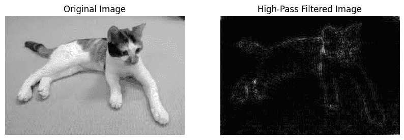
High-Pass Filtering

4. Image Compression

FFT-based image compression reduces image size by removing less important frequency components while preserving the main image features.

• The image is converted to the frequency domain using FFT.
• Low importance frequency components are removed.
• The remaining frequencies are converted back using the Inverse FFT.
• The compressed image uses less data but may lose some fine details, causing slight blurring.

You can download the image from here

Python `

import numpy as np import cv2 import matplotlib.pyplot as plt

image = cv2.imread('image path', cv2.IMREAD_GRAYSCALE)

f = np.fft.fft2(image) fshift = np.fft.fftshift(f)

threshold = 0.005 * np.max(np.abs(fshift)) fshift_compressed = np.where(np.abs(fshift) > threshold, fshift, 0)

f_ishift = np.fft.ifftshift(fshift_compressed) compressed_image = np.fft.ifft2(f_ishift) compressed_image = np.abs(compressed_image)

compressed_image = cv2.normalize( compressed_image, None, 0, 255, cv2.NORM_MINMAX ).astype(np.uint8)

plt.figure(figsize=(10, 5))

plt.subplot(1, 2, 1) plt.imshow(image, cmap='gray') plt.title("Original Image") plt.axis('off')

plt.subplot(1, 2, 2) plt.imshow(compressed_image, cmap='gray') plt.title("Compressed Image") plt.axis('off')

plt.show()

`

**Output:

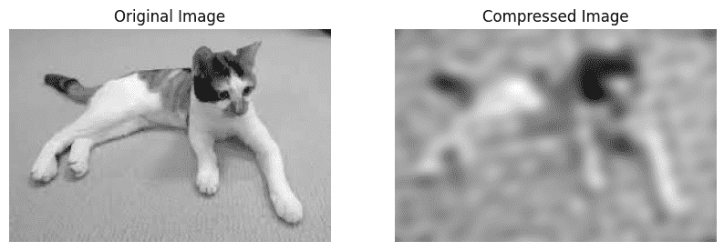
Compressed Image

5. Edge Detection

Edge detection highlights object boundaries and sharp intensity changes in an image by emphasizing high frequency components.

• The image is converted to the frequency domain using FFT.
• A Laplacian filter is applied to enhance edge information.
• The filtered frequency data is converted back using the Inverse FFT.
• The resulting image highlights edges and important structural details.

You can download the image from here

Python `

import numpy as np import cv2 import matplotlib.pyplot as plt

image = cv2.imread('/content/cat img.jpeg', cv2.IMREAD_GRAYSCALE)

f = np.fft.fft2(image)

laplacian = np.array([[0, 1, 0], [1, -4, 1], [0, 1, 0]])

kernel = np.zeros_like(image, dtype=np.float32) kernel[:3, :3] = laplacian

kernel_fft = np.fft.fft2(kernel)

filtered = f * kernel_fft

image_edge = np.abs(np.fft.ifft2(filtered))

image_edge = cv2.normalize( image_edge, None, 0, 255, cv2.NORM_MINMAX ).astype(np.uint8)

plt.figure(figsize=(10,5))

plt.subplot(121) plt.imshow(image, cmap='gray') plt.title("Original Image") plt.axis('off')

plt.subplot(122) plt.imshow(image_edge, cmap='gray') plt.title("Edge Detection") plt.axis('off')

plt.show()

`

**Output:

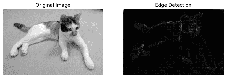
Edge Detection

**6. Pattern Recognition

Pattern recognition uses frequency domain correlation to identify whether a specific pattern or template exists within an image.

• The image and template are converted to the frequency domain using FFT.
• Correlation is computed between the image and template in the frequency domain.
• The correlation result is analyzed to find matching patterns.
• A threshold is used to determine whether the pattern is present in the image.
• If the correlation exceeds the threshold, the pattern is considered detected.

• You can download the image from here
• You can download the template from here

Python `

import numpy as np import cv2 import matplotlib.pyplot as plt

image = cv2.imread('image path', cv2.IMREAD_GRAYSCALE) template = cv2.imread('template path', cv2.IMREAD_GRAYSCALE)

image_fft = np.fft.fft2(image) template_fft = np.fft.fft2(template, s=image.shape)

correlation = np.fft.ifft2(image_fft * np.conj(template_fft)) correlation = np.abs(correlation)

max_corr = np.max(correlation) threshold = 0.8 * max_corr

if max_corr > threshold: print("Pattern detected in the image.") else: print("No pattern detected in the image.")

plt.figure(figsize=(15, 5))

plt.subplot(1, 3, 1) plt.imshow(image, cmap='gray') plt.title("Input Image") plt.axis('off')

plt.subplot(1, 3, 2) plt.imshow(template, cmap='gray') plt.title("Template Image") plt.axis('off')

plt.subplot(1, 3, 3) plt.imshow(correlation, cmap='hot') plt.title("Correlation Map") plt.colorbar() plt.axis('off')

plt.show()

`

**Output:

Pattern detected in the image

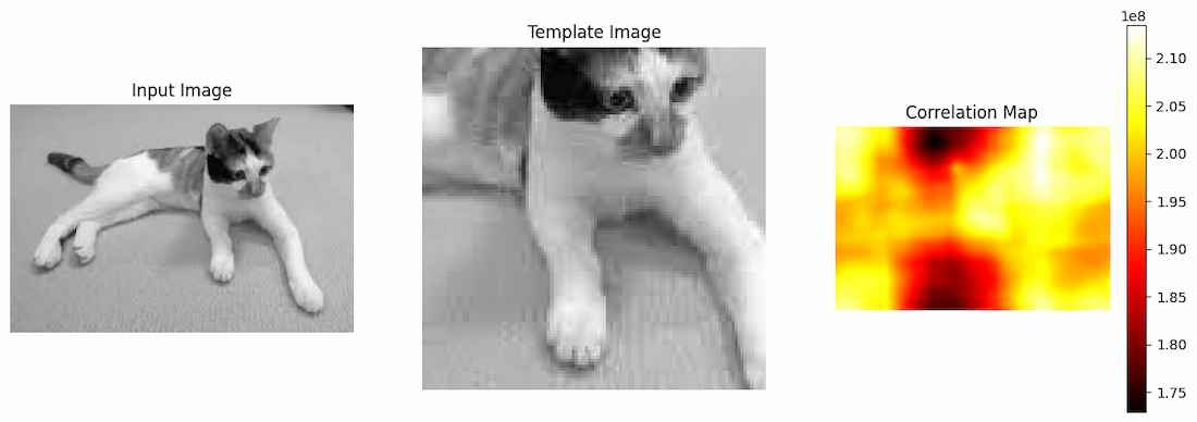
Pattern Recognition

**7. Blur Detection

Blur detection uses FFT to analyze the frequency content of an image. Blurred images contain fewer high-frequency components than sharp images.

• The image is converted to the frequency domain using FFT.
• High frequency energy is measured from the frequency spectrum.
• A threshold is used to classify the image as sharp or blurred.
• Lower high frequency energy usually indicates a blurred image.

You can download the image from here

Python `

import numpy as np import cv2 import matplotlib.pyplot as plt

image = cv2.imread('/content/cat img.jpeg', cv2.IMREAD_GRAYSCALE)

f = np.fft.fft2(image) fshift = np.fft.fftshift(f)

magnitude_spectrum = np.log(np.abs(fshift) + 1)

rows, cols = image.shape crow, ccol = rows // 2, cols // 2

mask = np.ones((rows, cols), np.uint8) mask[crow-20:crow+20, ccol-20:ccol+20] = 0

high_freq_energy = np.mean(magnitude_spectrum * mask)

print("High Frequency Energy:", round(high_freq_energy, 2))

threshold = 3.5

if high_freq_energy < threshold: print("The image is blurred.") else: print("The image is sharp.")

`

**Output:

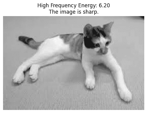
Sharp Image

Download full code from here

Advantages

• Enables efficient analysis of images in the frequency domain.
• Helps remove unwanted noise by filtering specific frequency components.
• Reduces storage requirements by retaining only significant frequency information.
• Assists in detecting patterns, edges and important image features.
• Improves image quality through enhancement and filtering operations.
• Performs frequency domain processing faster than traditional Fourier Transform methods.

Limitations

• Large images can require significant memory and computational resources.
• Removing important frequency components may reduce image quality.
• Frequency domain representations can be difficult to interpret compared to pixel based images.
• Selecting appropriate frequency filters often requires careful tuning.
• FFT is less effective when image features vary significantly across different regions.