Fast Fourier Transform (FFT) in SciPy (original) (raw)

Last Updated : 7 Jul, 2025

Fourier analysis is a scientific computing technique widely used in signal processing, image compression and numerical simulations. The idea is that any complex signal can be expressed as a combination of simple, periodic components like sine and cosine waves. This process of decomposition is called the **Fourier Transform.

The Fast Fourier Transform (FFT) is one algorithm that makes Fourier analysis practical for real-world applications. **SciPy is a core library for scientific computing in Python, offers a module called fftpack that allows users to perform these transformations efficiently. This article provides an overview of FFT using SciPy’s FFTPack.

Fourier Transform

A time-domain signal(Audio waveform) is a sequence of amplitude values over time. The Fourier Transform converts this into the frequency domain, showing what frequency components make up the signal. For example, a guitar string vibrating at multiple harmonics can be broken down into these individual frequencies.

In digital systems, we work with a sampled version of the signal. This discrete set of samples is transformed using the **Discrete Fourier Transform (DFT). The DFT is defined mathematically as:

X_k = \sum_{n=0}^{N-1} x_n \cdot e^{-2\pi i k n / N}, \quad 0 \leq k < N

x_n: The input signal or data sequence in the time domain
X_k**: The DCT output coefficient at frequency index k
N: Total number of input points (length of the input sequence)
n: Index variable over input time-domain samples (ranges from 0 to N−1 )
k: Index variable over frequency-domain coefficients (ranges from 0 to N−1)

Here, x_n is the input signal, and X_k is the transformed frequency component. Computing this directly for large N is computationally expensive. The **Fast Fourier Transform (FFT) reduces this complexity by using symmetries in the DFT formula.

Performing FFT with SciPy

SciPy’s FFTpack module provides a interface to compute both FFT and its inverse (IFFT). These functions accept NumPy arrays and return the transformed signal in complex number form.

FFT : Transforming Time to Frequency domain

Python `

from scipy.fftpack import fft import numpy as np

Create a time vector

t = np.linspace(0, 1, 100, endpoint=False) # 1 second, 100 samples

Composite signal: sine + cosine

x = np.sin(2 * np.pi * 5 * t) + 0.5 * np.cos(2 * np.pi * 10 * t)

Apply FFT

y = fft(x)

Print real and imaginary parts of first 10 frequency components

print("FFT Output (first 10 samples):") for i in range(10): print(f"Frequency bin {i}: {y[i].real:.2f} + {y[i].imag:.2f}j")

**Output:

FFT-transform

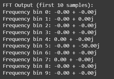
Frequency Outputs

IFFT: Reconstructing Signal and Plot

Python `

import matplotlib.pyplot as plt

Create a time vector

t = np.linspace(0, 1, 100, endpoint=False)

Composite signal: sine + cosine

x = np.sin(2 * np.pi * 5 * t) + 0.5 * np.cos(2 * np.pi * 10 * t)

FFT and inverse FFT

y = fft(x) x_reconstructed = ifft(y)

Print first 10 reconstructed values

print("Reconstructed signal (first 10 samples):", np.round(x_reconstructed.real[:10], 2))

Visualization

plt.figure(figsize=(10, 4))

Original signal

plt.subplot(1, 2, 1) plt.plot(t, x) plt.title("Original Signal") plt.xlabel("Time") plt.ylabel("Amplitude")

Reconstructed signal

plt.subplot(1, 2, 2) plt.plot(t, x_reconstructed.real) plt.title("Reconstructed Signal from IFFT") plt.xlabel("Time") plt.ylabel("Amplitude")

plt.tight_layout() plt.show()

**Output:

IFFT-transformed-values

Reconstructed Outputs

Original-vs-Reconstructed

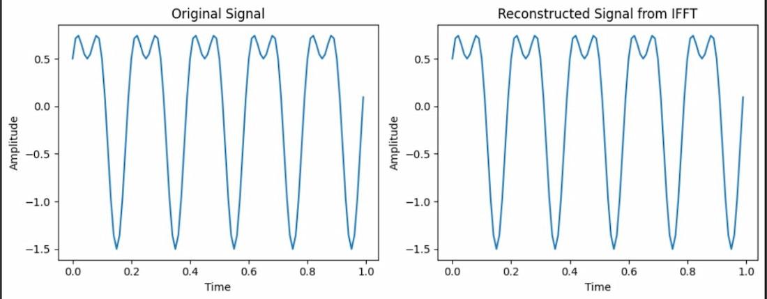
Original data vs Reconstructed data

This script shows both the transformation and the reconstruction. After applying FFT, the output is a list of complex numbers representing frequency amplitudes and phases. Applying IFFT reconstructs the original signal (within a margin of numerical error).

Considerations and Limitations

**Input Size: FFT is fastest when the number of input samples N is a power of 2, although modern implementations handle arbitrary sizes.
**Numerical Precision: Due to floating-point arithmetic, inverse transformations might not reproduce the exact input but will be close within machine precision.
**Complex Output: FFT outputs complex numbers even if the input is purely real. In practice, the imaginary parts are often negligible or symmetric.
**Dimensionality: The examples here are for 1D signals. SciPy also supports 2D and multi-dimensional FFTs (fft2, fftn), useful for image and volumetric data.

SciPy’s FFTpack makes frequency-domain analysis in Python accessible and efficient. It helps in working with sound signals, compressing images or analyzing time series data.