Principal Component Analysis (PCA) (original) (raw)

Last Updated : 15 Apr, 2026

PCA (Principal Component Analysis) is a dimensionality reduction technique and helps us to reduce the number of features in a dataset while keeping the most important information. It changes complex datasets by transforming correlated features into a smaller set of uncorrelated components.

Principal Component Analysis (PCA)

It helps us to remove redundancy, improve computational efficiency and make data easier to visualize and analyze.

How Principal Component Analysis Works

PCA uses linear algebra to transform data into new features called principal components. It finds these by calculating eigenvectors (directions) and eigenvalues (importance) from the covariance matrix. PCA selects the top components with the highest eigenvalues and projects the data onto them simplify the dataset.

**Note: _It prioritizes the directions where the data varies the most because more variation = more useful information.

Imagine you’re looking at a messy cloud of data points like stars in the sky and want to simplify it. PCA helps you find the "most important angles" to view this cloud so you don’t miss the big patterns. Here’s how it works step by step:

**Step 1: Standardize the Data

Different features may have different units and scales like salary vs. age. To compare them fairly PCA first standardizes the data by making each feature have:

• A mean of 0
• A standard deviation of 1

Z = \frac{X-\mu}{\sigma}

where:

• \mu is the mean of independent features \mu = \left \{ \mu_1, \mu_2, \cdots, \mu_m \right \}
• \sigma is the standard deviation of independent features \sigma = \left \{ \sigma_1, \sigma_2, \cdots, \sigma_m \right \}

**Step 2: Calculate Covariance Matrix

Next PCA calculates the covariance matrix to see how features relate to each other whether they increase or decrease together. The covariance between two features x_1 and x_2 is:

cov(x1,x2) = \frac{\sum_{i=1}^{n}(x1_i-\bar{x1})(x2_i-\bar{x2})}{n-1}

Where:

• \bar{x}_1 \,and \, \bar{x}_2​ are the mean values of features x_1 \, and\, x_2
• n is the number of data points

The value of covariance can be positive, negative or zeros.

**Step 3: Find the Principal Components

PCA identifies new axes where the data spreads out the most:

• **1st Principal Component (PC1): The direction of maximum variance (most spread).
• **2nd Principal Component (PC2): The next best direction, _perpendicular to PC1 and so on.

These directions come from the eigenvectors of the covariance matrix and their importance is measured by eigenvalues. For a square matrix A an eigenvector X (a non-zero vector) and its corresponding eigenvalue λ satisfy:

AX = \lambda X

This means:

• When _A acts on X it only stretches or shrinks X by the scalar λ.
• The direction of X remains unchanged hence eigenvectors define "stable directions" of A.

Eigenvalues help rank these directions by importance.

**Step 4: Pick the Top Directions & Transform Data

After calculating the eigenvalues and eigenvectors PCA ranks them by the amount of information they capture. We then:

1. Select the top k components that capture most of the variance like 95%.
2. Transform the original dataset by projecting it onto these top components.

This means we reduce the number of features (dimensions) while keeping the important patterns in the data.

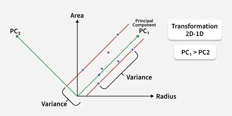
Transform this 2D dataset into a 1D representation while preserving as much variance as possible.

In the above image the original dataset has two features "Radius" and "Area" represented by the black axes. PCA identifies two new directions: PC₁ and PC₂ which are the principal components.

• These new axes are rotated versions of the original ones. PC₁ captures the maximum variance in the data meaning it holds the most information while PC₂ captures the remaining variance and is perpendicular to PC₁.
• The spread of data is much wider along PC₁ than along PC₂. This is why PC₁ is chosen for dimensionality reduction. By projecting the data points (blue crosses) onto PC₁ we effectively transform the 2D data into 1D and retain most of the important structure and patterns.

Implementation of Principal Component Analysis in Python

Hence PCA uses a linear transformation that is based on preserving the most variance in the data using the least number of dimensions. It involves the following steps:

**Step 1: Importing Required Libraries

We import the necessary library like pandas, numpy, scikit learn, seaborn and matplotlib to visualize results.

Python `

import numpy as np import pandas as pd from sklearn.preprocessing import StandardScaler from sklearn.decomposition import PCA from sklearn.model_selection import train_test_split from sklearn.linear_model import LogisticRegression from sklearn.metrics import confusion_matrix import matplotlib.pyplot as plt import seaborn as sns

`

Step 2: Creating Sample Dataset

We make a small dataset with three features Height, Weight, Age and Gender.

Python `

data = { 'Height': [170, 165, 180, 175, 160, 172, 168, 177, 162, 158], 'Weight': [65, 59, 75, 68, 55, 70, 62, 74, 58, 54], 'Age': [30, 25, 35, 28, 22, 32, 27, 33, 24, 21], 'Gender': [1, 0, 1, 1, 0, 1, 0, 1, 0, 0] # 1 = Male, 0 = Female } df = pd.DataFrame(data) print(df)

`

**Output:

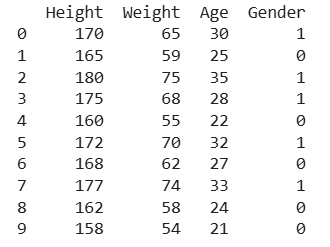
Dataset

Step 3: Standardizing the Data

Since the features have different scales Height vs Age we standardize the data. This makes all features have mean = 0 and standard deviation = 1 so that no feature dominates just because of its units.

Python `

X = df.drop('Gender', axis=1) y = df['Gender']

scaler = StandardScaler() X_scaled = scaler.fit_transform(X)

`

Step 4: Applying PCA algorithm

• We reduce the data from 3 features to 2 new features called principal components. These components capture most of the original information but in fewer dimensions.
• We split the data into 70% training and 30% testing sets.
• We train a logistic regression model on the reduced training data and predict gender labels on the test set. Python `

pca = PCA(n_components=2) X_pca = pca.fit_transform(X_scaled)

X_train, X_test, y_train, y_test = train_test_split(X_pca, y, test_size=0.3, random_state=42)

model = LogisticRegression() model.fit(X_train, y_train)

y_pred = model.predict(X_test)

`

Step 5: Evaluating with Confusion Matrix

The confusion matrix compares actual vs predicted labels. This makes it easy to see where predictions were correct or wrong.

Python `

cm = confusion_matrix(y_test, y_pred)

plt.figure(figsize=(5,4)) sns.heatmap(cm, annot=True, fmt='d', cmap='Blues', xticklabels=['Female', 'Male'], yticklabels=['Female', 'Male']) plt.xlabel('Predicted Label') plt.ylabel('True Label') plt.title('Confusion Matrix') plt.show()

`

**Output:

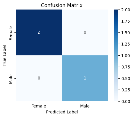
Confusion matrix

Step 6: Visualizing PCA Result

Python `

y_numeric = pd.factorize(y)[0]

plt.figure(figsize=(12, 5))

plt.subplot(1, 2, 1) plt.scatter(X_scaled[:, 0], X_scaled[:, 1], c=y_numeric, cmap='coolwarm', edgecolor='k', s=80) plt.xlabel('Original Feature 1') plt.ylabel('Original Feature 2') plt.title('Before PCA: Using First 2 Standardized Features') plt.colorbar(label='Target classes')

plt.subplot(1, 2, 2) plt.scatter(X_pca[:, 0], X_pca[:, 1], c=y_numeric, cmap='coolwarm', edgecolor='k', s=80) plt.xlabel('Principal Component 1') plt.ylabel('Principal Component 2') plt.title('After PCA: Projected onto 2 Principal Components') plt.colorbar(label='Target classes')

plt.tight_layout() plt.show()

`

**Output:

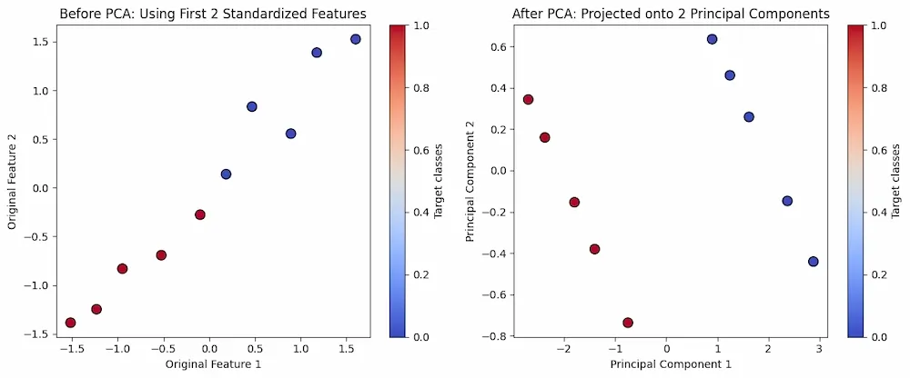
PCA Algorithm

• **Left Plot Before PCA: This shows the original standardized data plotted using the first two features. There is no guarantee of clear separation between classes as these are raw input dimensions.
• **Right Plot After PCA: This displays the transformed data using the top 2 principal components. These new components capture the maximum variance often showing better class separation and structure making it easier to analyze or model.

You can download source code from here.

**Advantages of Principal Component Analysis

1. **Multicollinearity Handling: Creates new, uncorrelated variables to address issues when original features are highly correlated.
2. **Noise Reduction: Eliminates components with low variance enhance data clarity.
3. **Data Compression: Represents data with fewer components reduce storage needs and speeding up processing.
4. **Outlier Detection: Identifies unusual data points by showing which ones deviate significantly in the reduced space.

**Disadvantages of Principal Component Analysis

1. **Interpretation Challenges: The new components are combinations of original variables which can be hard to explain.
2. **Data Scaling Sensitivity: Requires proper scaling of data before application or results may be misleading.
3. **Information Loss: Reducing dimensions may lose some important information if too few components are kept.
4. **Assumption of Linearity: Works best when relationships between variables are linear and may struggle with non-linear data.
5. **Computational Complexity: Can be slow and resource-intensive on very large datasets.