Understanding the Confusion Matrix in Machine Learning (original) (raw)
Last Updated : 23 Jan, 2026
Confusion matrix is a simple table used to measure how well a classification model is performing. It compares the predictions made by the model with the actual results and shows where the model was right or wrong. This helps you understand where the model is making mistakes so you can improve it. It breaks down the predictions into four categories:
- **True Positive (TP): The model correctly predicted a positive outcome i.e the actual outcome was positive.
- **True Negative (TN): The model correctly predicted a negative outcome i.e the actual outcome was negative.
- **False Positive (FP): The model incorrectly predicted a positive outcome i.e the actual outcome was negative. It is also known as a Type I error.
- **False Negative (FN): The model incorrectly predicted a negative outcome i.e the actual outcome was positive. It is also known as a Type II error.

Confusion Matrix
It also helps calculate key measures like **accuracy, **precision and **recall which give a better idea of performance especially when the data is imbalanced.
Metrics based on Confusion Matrix Data
1. Accuracy
Accuracy shows how many predictions the model got right out of all the predictions. It gives idea of overall performance but it can be misleading when one class is more dominant over the other. For example a model that predicts the majority class correctly most of the time might have high accuracy but still fail to capture important details about other classes. It can be calculated using the below formula:
\text{Accuracy} = \frac {TP+TN}{TP+TN+FP+FN}
2. Precision
Precision focus on the quality of the model’s positive predictions. It tells us how many of the "positive" predictions were actually correct. It is important in situations where false positives need to be minimized such as detecting spam emails or fraud. The formula of precision is:
\text{Precision} = \frac{TP}{TP+FP}
3. Recall
Recall measures how how good the model is at predicting positives. It shows the proportion of true positives detected out of all the actual positive instances. High recall is essential when missing positive cases has significant consequences like in medical tests.
\text{Recall} = \frac{TP}{TP+FN}
4. F1-Score
F1-score combines precision and recall into a single metric to balance their trade-off. It provides a better sense of a model’s overall performance particularly for imbalanced datasets. It is helpful when both false positives and false negatives are important though it assumes precision and recall are equally important but in some situations one might matter more than the other.
\text{F1-Score} = \frac {2 \cdot Precision \cdot Recall}{Precision + Recall}
5. Specificity
Specificity is another important metric in the evaluation of classification models particularly in binary classification. It measures the ability of a model to correctly identify negative instances. Specificity is also known as the True Negative Rate Formula is given by:
\text{Specificity} = \frac{TN}{TN+FP}
**6. Type 1 and Type 2 error
Type 1 and Type 2 error are:
- **Type 1 error: It occurs when the model incorrectly predicts a positive instance but the actual instance is negative. This is also known as a **false positive. Type 1 Errors affect the **precision of a model which measures the accuracy of positive predictions.
\text{Type 1 Error} = \frac{\text{FP}}{\text{FP} + \text{TN}}
- **Type 2 error: This occurs when the model fails to predict a positive instance even though it is actually positive. This is also known as a **false negative. Type 2 Errors impact the **recall of a model which measures how well the model identifies all actual positive cases.
\text{Type 2 Error} = \frac{FN}{TP+FN}
**Example: A diagnostic test is used to detect a particular disease in patients.
- **Type 1 Error (False Positive): This occurs when the test predicts a patient has the disease (positive result) but the patient is actually healthy (negative case).
- **Type 2 Error (False Negative): This occurs when the test predicts the patient is healthy (negative result) but the patient actually has the disease (positive case).
Confusion Matrix For Binary Classification
A 2x2 Confusion matrix is shown below for the image recognition having a Dog image or Not Dog image:
| Predicted | Predicted | |
|---|---|---|
| Actual | True Positive (TP) | False Negative (FN) |
| Actual | False Positive (FP) | True Negative (TN) |
- **True Positive (TP): It is the total counts having both predicted and actual values are Dog.
- **True Negative (TN): It is the total counts having both predicted and actual values are Not Dog.
- **False Positive (FP): It is the total counts having prediction is Dog while actually Not Dog.
- **False Negative (FN): It is the total counts having prediction is Not Dog while actually, it is Dog.
Example: Confusion Matrix for Dog Image Recognition with Numbers
| Index | 1 | 2 | 3 | 4 | 5 | 6 | 7 | 8 | 9 | 10 |
|---|---|---|---|---|---|---|---|---|---|---|
| Actual | Dog | Dog | Dog | Not Dog | Dog | Not Dog | Dog | Dog | Not Dog | Not Dog |
| Predicted | Dog | Not Dog | Dog | Not Dog | Dog | Dog | Dog | Dog | Not Dog | Not Dog |
| Result | TP | FN | TP | TN | TP | FP | TP | TP | TN | TN |
- Actual Dog Counts = 6
- Actual Not Dog Counts = 4
- True Positive Counts = 5
- False Positive Counts = 1
- True Negative Counts = 3
- False Negative Counts = 1
| Predicted | |||
|---|---|---|---|
| Dog | Not Dog | ||
| Actual | Dog | True Positive(TP =5) | False Negative(FN =1) |
| Not Dog | False Positive(FP=1) | True Negative(TN=3) |
Implementation of Confusion Matrix for Binary classification using Python
**Step 1: Import the necessary libraries
Python `
import numpy as np from sklearn.metrics import confusion_matrix,classification_report import seaborn as sns import matplotlib.pyplot as plt
`
**Step 2: Create the NumPy array for actual and predicted labels
- **actual: represents the true labels or the actual classification of the items. In this case it's a list of 10 items where each entry is either 'Dog' or 'Not Dog'.
- **predicted: represents the predicted labels or the classification made by the model. Python `
actual = np.array( ['Dog','Dog','Dog','Not Dog','Dog','Not Dog','Dog','Dog','Not Dog','Not Dog']) predicted = np.array( ['Dog','Not Dog','Dog','Not Dog','Dog','Dog','Dog','Dog','Not Dog','Not Dog'])
`
**Step 3: Compute the confusion matrix
- **confusion_matrix: This function from sklearn.metrics computes the confusion matrix which is a table used to evaluate the performance of a classification algorithm. It compares actual and predicted to generate a matrix Python `
cm = confusion_matrix(actual,predicted)
`
**Step 4: Plot the confusion matrix with the help of the seaborn heatmap
- **sns.heatmap: This function from **Seaborn is used to create a heatmap of the confusion matrix.
- **annot=True: Display the numerical values in each cell of the heatmap. Python `
sns.heatmap(cm, annot=True, fmt='g', xticklabels=['Dog','Not Dog'], yticklabels=['Dog','Not Dog']) plt.ylabel('Actual', fontsize=13) plt.title('Confusion Matrix', fontsize=17, pad=20) plt.gca().xaxis.set_label_position('top') plt.xlabel('Prediction', fontsize=13) plt.gca().xaxis.tick_top()
plt.gca().figure.subplots_adjust(bottom=0.2) plt.gca().figure.text(0.5, 0.05, 'Prediction', ha='center', fontsize=13) plt.show()
`
**Output:

Visualizing the Confusion Matrix
**Step 5: Classifications Report based on Confusion Metrics
Python `
print(classification_report(actual, predicted))
`
**Output:
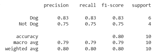
Classification Report
Confusion Matrix For Multi-class Classification
In **multi-class classification the confusion matrix is expanded to account for multiple classes.
- **Rows represent the actual classes (ground truth).
- **Columns represent the predicted classes.
- Each cell in the matrix shows how often a specific actual class was predicted as another class.
For example in a 3-class problem the confusion matrix would be a 3x3 table where each row and column corresponds to one of the classes. It summarizes the model's performance across all classes in a compact format. Lets consider the below example:
Example: Confusion Matrix for Image Classification (Cat, Dog, Horse)
| Actual\Predicted | Predicted Cat | Predicted Dog | Predicted Horse |
|---|---|---|---|
| **Actual Cat | Correct | Misclassified | Misclassified |
| **Actual Dog | Misclassified | Correct | Misclassified |
| **Actual Horse | Misclassified | Misclassified | Correct |
**Note: In multi-class classification, off-diagonal values represent misclassifications.
For a given class, a misclassified instance acts as a False Negative (FN) for the actual class and a False Positive (FP) for the predicted class. Therefore, FP and FN are defined per class, not per cell.
**Example with Numbers:
When evaluating one class at a time (one-vs-rest), the confusion matrix metrics such as TP, FP, FN and TN are calculated separately for each class. Let's consider the scenario where the model processed 30 images:
| Predicted Cat | Predicted Dog | Predicted Horse | |
|---|---|---|---|
| Actual Cat | 8 | 1 | 1 |
| Actual Dog | 2 | 10 | 0 |
| Actual Horse | 0 | 2 | 8 |
In this scenario:
- **Cats: 8 were correctly identified, 1 was misidentified as a dog and 1 was misidentified as a horse.
- **Dogs: 10 were correctly identified, 2 were misidentified as cats.
- **Horses: 8 were correctly identified, 2 were misidentified as dogs.
To calculate true negatives, we need to know the total number of images that were NOT cats, dogs or horses. Let's assume there were 10 such images and the model correctly classified all of them as "not cat," "not dog," and "not horse." Therefore:
- **True Negative (TN) Counts: 10 for each class as the model correctly identified each non-cat/dog/horse image as not belonging to that class
Implementation of Confusion Matrix for Multi-Class classification using Python
**Step 1: Import the necessary libraries
Python `
import numpy as np from sklearn.metrics import confusion_matrix, ConfusionMatrixDisplay, classification_report import matplotlib.pyplot as plt
`
**Step 2: Create the NumPy array for actual and predicted labels
- **y_true: List of true labels.
- **y_pred: List of predicted labels by the model.
- **classes: A list of class names: 'Cat', 'Dog' and 'Horse' Python `
y_true = ['Cat'] * 10 + ['Dog'] * 12 + ['Horse'] * 10 y_pred = ['Cat'] * 8 + ['Dog'] + ['Horse'] + ['Cat'] * 2 + ['Dog'] * 10 + ['Horse'] * 8 + ['Dog'] * 2 classes = ['Cat', 'Dog', 'Horse']
`
**Step 3: Generate and Visualize the Confusion Matrix
- **ConfusionMatrixDisplay: Creates a display object for the confusion matrix.
- **confusion_matrix=cm: Passes the confusion matrix (
cm) to display. - **display_labels=classes: Sets the labels (['Cat' , 'Dog' , 'Horse']) or the confusion matrix. Python `
cm = confusion_matrix(y_true, y_pred, labels=classes) disp = ConfusionMatrixDisplay(confusion_matrix=cm, display_labels=classes) disp.plot(cmap=plt.cm.Blues) plt.title('Confusion Matrix', fontsize=15, pad=20) plt.xlabel('Prediction', fontsize=11) plt.ylabel('Actual', fontsize=11) plt.gca().xaxis.set_label_position('top') plt.gca().xaxis.tick_top() plt.gca().figure.subplots_adjust(bottom=0.2) plt.gca().figure.text(0.5, 0.05, 'Prediction', ha='center', fontsize=13)
plt.show()
`
**Output:

Display the confusion matrix
**Step 4: Print the Classification Report
Python `
print(classification_report(y_true, y_pred, target_names=classes))
`
**Output:
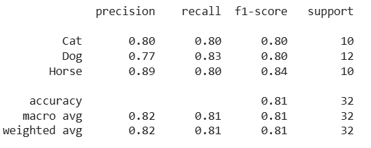
Classification Report
Confusion matrix provides clear insights into important metrics like accuracy, precision and recall by analyzing correct and incorrect predictions.