Data Cleaning (original) (raw)

Last Updated : 28 Apr, 2026

Data cleaning is the process of preparing raw data by detecting and correcting errors so it can be effectively used for analysis. It is a foundational step in data preprocessing that ensures datasets are suitable for analytical, statistical and machine learning tasks.

• Raw data is often noisy, incomplete and inconsistent which can negatively impact the accuracy of the model.
• Clean datasets are also important in EDA (Exploratory Data Analysis), which enhances the interpretability of data so that the right actions can be taken based on insights.

Common Data Anomalies

Data quality issues can arise from human errors, system failures or problems during data collection and integration. Some of the most common data quality challenges include:

• **Missing values: Incomplete records can reduce statistical power and introduce bias into analysis.
• **Duplicate records: Repeated entries may overrepresent certain observations resulting in skewed outcomes.
• **Incorrect data types: Mismatched formats, such as text stored in numeric fields can cause calculation errors and analysis failures.
• **Outliers and anomalies: Extremely high or low values can distort statistical measures and influence model performance.
• **Inconsistent formats: Variations in date formats, text casing or measurement units can create issues when merging or comparing datasets.
• **Spelling and typographical errors: Errors in text fields can lead to incorrect grouping, classification or interpretation of categorical data

Data Cleaning Process

1. Assess Data Quality

The first step in data cleaning is to assess the quality of your data. This involves checking for:

• **Missing Values: Identify any blank or null values in the dataset. Missing values can be due to various reasons such as incomplete data collection, data entry errors or data loss during transmission.
• **Incorrect Values: Check for values that are outside the expected range or are inconsistent with the data type.
• **Inconsistencies in Data Format: Verify that the data format is consistent throughout the dataset.

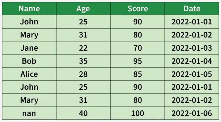
Imperfect Dataframe

After assessing data quality, several issues can be identified in the dataset:

• Rows 1 and 6 are duplicates indicating potential data duplication that may distort analysis.
• Row 7 has a missing value in the "Name" column, which could impact calculations or summaries.
• The "Date" column uses the "YYYY-MM-DD" format, but it is important to maintain this consistency across all entries.
• The score of 100 in row 7 may be an outlier depending on the scoring system, which could skew statistical analysis.

2. Remove Irrelevant Data

Removing irrelevant or duplicate data ensures the dataset is clean, accurate and meaningful, preventing skewed analysis and improving overall quality.

• Identify duplicate entries using techniques like sorting, grouping or hashing.
• Remove duplicate records to ensure each data point is unique and correctly represented.
• Detect redundant observations that do not add new information to the dataset.
• Eliminate variables or columns that are irrelevant to the analysis and do not provide useful insights.

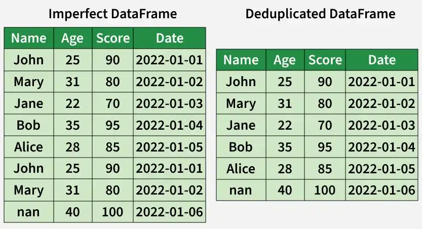
Remove Irrelevant Data

In the deduplicated DataFrame, the duplicate rows 1 and 6 have been removed to ensure each record is unique

3. Fix Structural Errors

Structural errors occur when data formats, naming conventions or variable types are inconsistent which can affect analysis accuracy. Correcting these issues ensures uniform and reliable data representation.

• Standardize data formats to maintain consistency in dates, times and other data types across the dataset.
• Correct naming inconsistencies in column names, variable names or labels to ensure clarity and uniformity.
• Ensure consistent data representation such as using the same units for measurements or the same scales for ratings.

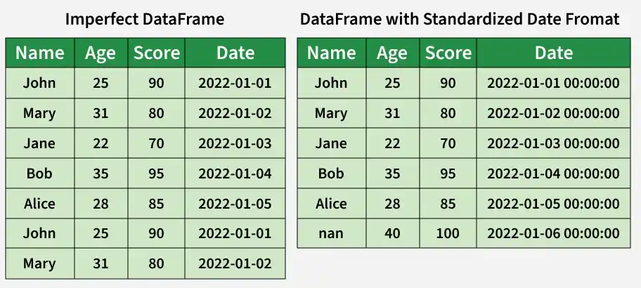
Fix Structural Errors

4. Handle Missing Data

Missing data can introduce bias and reduce the reliability of analysis. Properly addressing missing values helps maintain the integrity of your dataset.

• Impute missing values using statistical methods such as mean, median or mode to fill gaps.
• Remove records with missing values when the missing data is extensive or cannot be accurately imputed.
• Apply advanced imputation techniques like regression, k-nearest neighbors or decision trees to estimate missing values.

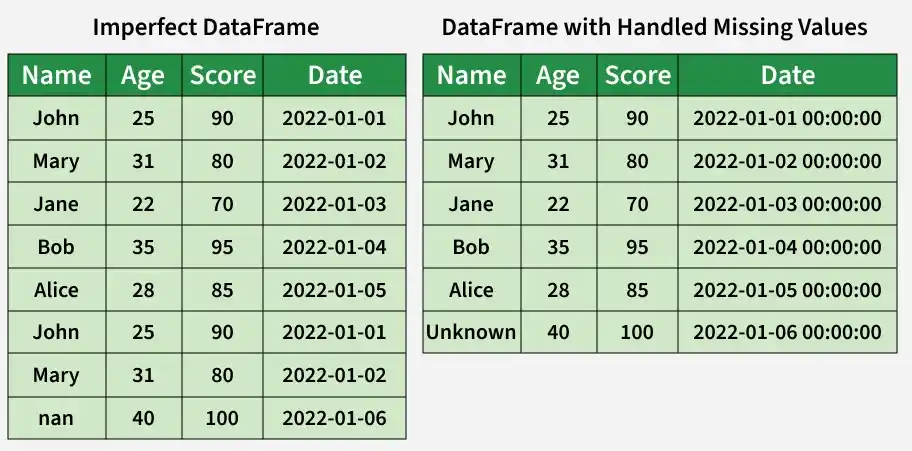
Handle Missing Data

The missing value in the 'Name' column (row 7) has been filled with 'Unknown' to indicate unavailable data, ensuring the dataset remains complete and consistent.

5. Normalize Data

Data normalization organizes the dataset to reduce redundancy and ensure consistency making it easier to manage and analyze.

• Split data into multiple tables, with each table storing specific types of information.
• Ensure consistency across the dataset to support efficient querying and accurate analysis.

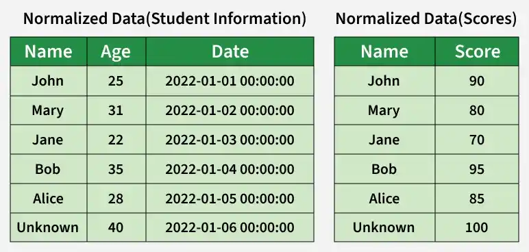
Normalize Data

6. Identify and Manage Outliers

Outliers are data points that deviate significantly from the rest of the dataset and can affect analysis accuracy. Properly handling them ensures more reliable insights.

• Remove outliers that result from errors or are not representative of the population.
• Transform extreme but valid outliers to reduce their impact on the analysis.

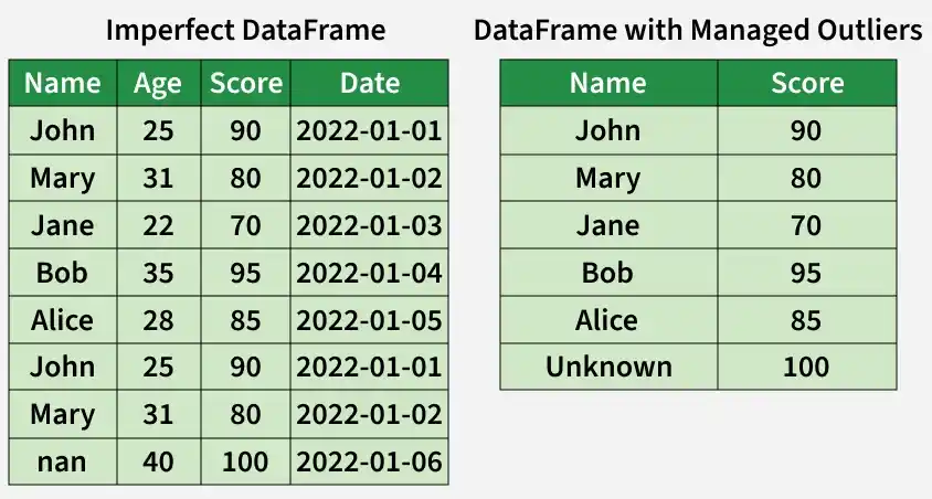
Manage Outliers

Implementation for Data Cleaning

Let's understand each step for Database Cleaning using titanic dataset.

You can download the dataset from here.

Step 1: Import Libraries and Load Dataset

We will import all the necessary libraries i.e pandas and numpy.

Python `

import pandas as pd import numpy as np

df = pd.read_csv('Titanic-Dataset.csv') df.info() df.head()

`

**Output:

Step 2: Check for Duplicate Rows

• **df.duplicated(): Returns a boolean Series indicating duplicate rows. Python `

df.duplicated()

`

**Output:

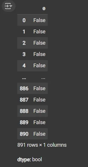
Duplicated Data

Step 3: Identify Column Data Types

• List comprehension with .dtype attribute to separate categorical and numerical columns.
• **object dtype: Generally used for text or categorical data. Python `

cat_col = [col for col in df.columns if df[col].dtype == 'object'] num_col = [col for col in df.columns if df[col].dtype != 'object']

print('Categorical columns:', cat_col) print('Numerical columns:', num_col)

`

**Output:

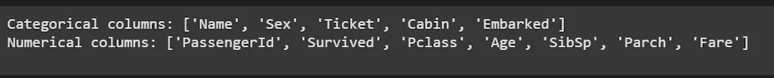
Column Data Types

Step 4: Count Unique Values in the Categorical Columns

• **df[cat_col].nunique(): Returns count of unique values per column. Python `

df[cat_col].nunique()

`

**Output:

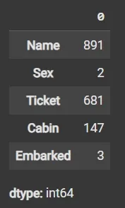
Unique Values

Step 5: Calculate Missing Values as Percentage

• **df.isnull(): Detects missing values, returning boolean DataFrame.
• Sum missing across columns, normalize by total rows and multiply by 100. Python `

round((df.isnull().sum() / df.shape[0]) * 100, 2)

`

**Output:

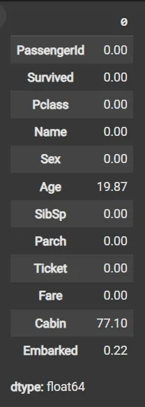
Missing Value Percentage

Step 6: Drop Irrelevant or Data-Heavy Missing Columns

• **df.drop(columns=[]): Drops specified columns from the DataFrame.
• **df.dropna(subset=[]): Removes rows where specified columns have missing values.
• **fillna(): Fills missing values with specified value (e.g., mean). Python `

df1 = df.drop(columns=['Name', 'Ticket', 'Cabin']) df1.dropna(subset=['Embarked'], inplace=True) df1['Age'] = df1['Age'].fillna(df1['Age'].mean())

`

Step 7: Detect Outliers with Box Plot

• **matplotlib.pyplot.boxplot(): Displays distribution of data, highlighting median, quartiles and outliers.
• **plt.show(): Renders the plot. Python `

import matplotlib.pyplot as plt

plt.boxplot(df1['Age'], vert=False) plt.ylabel('Variable') plt.xlabel('Age') plt.title('Box Plot') plt.show()

`

**Output:

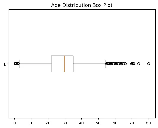
Boxplot

Step 8: Calculate Outlier Boundaries and Remove Them

• Calculate mean and standard deviation (std) using df['Age'].mean() and df['Age'].std().
• Define bounds as mean ± 2 * std for outlier detection.
• Filter DataFrame rows within bounds using Boolean indexing. Python `

mean = df1['Age'].mean() std = df1['Age'].std()

lower_bound = mean - 2 * std upper_bound = mean + 2 * std

df2 = df1[(df1['Age'] >= lower_bound) & (df1['Age'] <= upper_bound)]

`

Step 9: Impute Missing Data Again if Any

**fillna() applied again on filtered data to handle any remaining missing values.

Python `

df3 = df2.fillna(df2['Age'].mean()) df3.isnull().sum()

`

**Output:

Missing Value

Step 10: Recalculate Outlier Bounds and Remove Outliers from the Updated Data

• **mean = df3['Age'].mean(): Calculates the average (mean) value of the Age column in the DataFrame df3.
• **std = df3['Age'].std(): Computes the standard deviation (spread or variability) of the Age column in df3.
• **lower_bound = mean - 2 * std: Defines the lower limit for acceptable Age values, set as two standard deviations below the mean.
• **upper_bound = mean + 2 * std: Defines the upper limit for acceptable Age values, set as two standard deviations above the mean.
• **df4 = df3[(df3['Age'] >= lower_bound) & (df3['Age'] <= upper_bound)]: Creates a new DataFrame df4 by selecting only rows where the Age value falls between the lower and upper bounds, effectively removing outlier ages outside this range. Python `

mean = df3['Age'].mean() std = df3['Age'].std()

lower_bound = mean - 2 * std upper_bound = mean + 2 * std

print('Lower Bound :', lower_bound) print('Upper Bound :', upper_bound)

df4 = df3[(df3['Age'] >= lower_bound) & (df3['Age'] <= upper_bound)]

`

**Output:

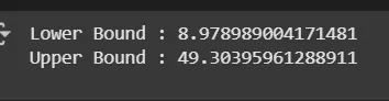
Outlier Check

Step 11: Data validation and verification

Data validation and verification involve ensuring that the data is accurate and consistent by comparing it with external sources or expert knowledge.

• For the machine learning prediction we separate independent and target features
• Here we will consider 'Pclass', 'Sex', 'Age', 'SibSp', 'Parch', 'Fare', and 'Embarked' as independent features.
• Survived as target variables because PassengerId will not affect the survival rate Python `

X = df3[['Pclass','Sex','Age', 'SibSp','Parch','Fare','Embarked']] Y = df3['Survived']

`

Step 12: Data formatting

Data formatting involves converting the data into a standard format or structure that can be easily processed by the algorithms or models used for analysis. Here we will discuss commonly used data formatting techniques i.e. Scaling and Normalization.

**1. Min-Max Scaling: Scaling involves transforming the values of features to a specific range. Min-Max scaling rescales the values to a specified range, typically between 0 and 1. It preserves the original distribution and ensures that the minimum value maps to 0 and the maximum value maps to 1.

Python `

from sklearn.preprocessing import MinMaxScaler

scaler = MinMaxScaler(feature_range=(0, 1))

num_col_ = [col for col in X.columns if X[col].dtype != 'object'] x1 = X x1[num_col_] = scaler.fit_transform(x1[num_col_]) x1.head()

`

**Output:

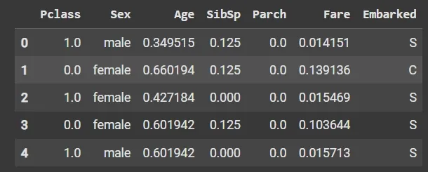
Min-Max Scaling

**2. Standardization (Z-score scaling): Standardization transforms the values to have a mean of 0 and a standard deviation of 1. It centers the data around the mean and scales it based on the standard deviation. Standardization makes the data more suitable for algorithms that assume a Gaussian distribution or require features to have zero mean and unit variance.

Z = (X - μ) / σ

Where,

• X = Data
• μ = Mean value of X
• σ = Standard deviation of X

You can download the source code from here.

Data Cleaning Strategies

• **Understand the data: Know the source, structure and domain of the data to identify potential quality issues and determine appropriate cleaning actions.
• **Document the process: Keep records of decisions, methods, assumptions and rules applied during data cleaning.
• **Prioritize critical issues: Focus first on major quality problems that could have a systemic impact on analysis or decision-making.
• **Automate where possible: Use scripts or tools for repetitive cleaning tasks to improve efficiency and consistency.
• **Collaborate with domain experts: Engage stakeholders or domain specialists to validate that the cleaned data meets business requirements.
• **Monitor and maintain: Continuously track data quality and perform cleaning periodically to ensure long-term accuracy and reliability.

Advantages

• Removing errors, inconsistencies, and irrelevant data helps the model learn better from the data.
• Ensures the data is accurate, consistent, and free of errors.
• Transforms data into a format that better represents underlying patterns and relationships.
• Improves data quality, making it more reliable and accurate.
• Helps identify and remove sensitive or confidential information, improving data security.

Disadvantages

• It is time-consuming, especially for large and complex datasets.
• It can lead to loss of important information if not handled carefully.
• Requires significant time, effort, expertise, and sometimes specialized tools.
• Removing too much data can contribute to underfitting.