Bernoulli Distribution in Statistics (original) (raw)
Last Updated : 23 Feb, 2026
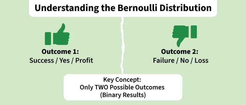
The Bernoulli Distribution is one of the most basic probability models used in statistics. It is designed to analyze situations where there are only two possible outcomes, such as success or failure, yes or no, profit or loss. This makes it extremely useful in business analytics because many real world decisions and performance metrics can be simplified into binary results.
Bernoulli Distribution
**It is based on the following assumptions:
- **Binary Outcomes Only: Exactly two outcomes Success (1) and Failure (0).
- **Probability of Success (p): Success probability = p; Failure probability = (1 − p).
- **Single Trial Model: Applied to one experiment or one observation at a time.
- **Expected Value (Mean): The expected value of a Bernoulli random variable is p. In business terms, this represents the average success rate over time.
- **Variance: The variance is p (1 − p). This measures the variability or uncertainty in the outcome.
Bernoulli Trial
A Bernoulli trial is a single experiment that results in only two possible outcomes: success (1) or failure (0). Each trial has a probability of success p and a probability of failure q = 1-p. A Bernoulli Distribution models the outcome of one such Bernoulli trial. In other words, the distribution provides the probability structure for a single success/failure experiment.
**Examples
- Flipping a coin (Heads = 1, Tails = 0)
- A customer clicking an ad (Click = 1, No Click = 0)
- A product passing inspection (Pass = 1, Fail = 0)
Conditions of Bernoulli Trials
- **Two possible outcomes: Each trial results in success or failure.
- **Constant probability: The probability of success p remains the same in every trial.
- **Independence: The outcome of one trial does not affect others.
- **Fixed number of trials: The number of repetitions is predetermined.
Bernoulli Distribution Graph
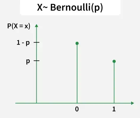
The Bernoulli Distribution is represented by a discrete probability graph with only two possible values on the horizontal axis: 0 and 1. Since the random variable can take only these two outcomes, the graph contains exactly two vertical bars (or spikes).
- At x = 0 , The height of the bar is 1-p this represents the probability of failure.
- At x = 1 , The height of the bar is p this represents the probability of success.
- The vertical axis shows P (X = x), which indicates the probability of each outcome.
Graph
Bernoulli Distribution Formulas
The Bernoulli Distribution formula is used to describe the probability of two possible outcomes:
- 1 : Success
- 0 : Failure
It is written as:
X \sim \text{Bernoulli}(p)
where:
- p: probability of success
- 1-p : probability of failure and
- 0 \leq p \leq 1
1. Probability Mass Function (PMF) for Bernoulli Distribution
The PMF gives the probability that the random variable X takes a specific value (0 or 1).
P(X = x) = p^x (1 - p)^{1 - x}, \quad x \in \{0,1\}, \quad 0 < p < 1
Here,
- If x = 1 then P(X = 1) = p (Probability of success)
- If x = 0 then P(X = 0) = 1-p (Probability of failure)
2. Cumulative Distribution Function for Bernoulli Distribution
The CDF gives the probability that the random variable X is less than or equal to a specific value.
F_X(x) =\begin{cases}0, & x < 0 \\1 - p, & 0 \leq x < 1 \\1, & x \geq 1\end{cases}
Here: The CDF increases in steps because a Bernoulli variable can take only two values: 0 and 1.
- If x<0: Probability is 0.
- If 0\leq x <1 : Probability is 1-p (only failure counted).
- If x \geq 1: Probability is 1 (both failure and success counted).
- The graph jumps at 0 and 1, showing that it is a discrete distribution.
**Example
Find the probability of getting heads (success) on flipping a fair coin.
**Solution: Let X represent the outcome of the coin toss.
X = 1 if heads, X = 0 if tails.
p (probability of success) is 0.5 for a fair coin and q (probability of failure) = 1 - p is 0.5
p = 0.5.
Bernoulli Distribution Metrics
1. Mean (μ) of Bernoulli Distribution
The mean of a Bernoulli distribution, also called the expected value, represents the long run average outcome of repeated independent trials. Since a Bernoulli variable takes only two values 1 (success) and 0 (failure), its mean is simply the probability of success.
In simple terms, if the probability of success is p = 0.5, then over many trials the average outcome will approach 0.5. The mean directly reflects how likely success is in a single trial.
For a Bernoulli random variable X:
- P(X = 1) = p \quad \text{(Success)}
- P(X = 0) = 1 - p \quad \text{(Failure)}
The expected value (mean) is calculated by multiplying each outcome by its probability and adding them:
E[X] = (1 \cdot p) + (0 \cdot (1 - p))
Final Result:
\mu = E[X] = p
2. Variance (σ2) of Bernoulli Distribution
Variance measures how much the two possible outcomes (0 and 1) deviate from the mean. For a Bernoulli distribution, the variance is p(1-p), meaning it depends entirely on the probability of success p and failure 1-p. Variability is highest when p = 0.5, because success and failure are equally likely. When p is close to 0 or 1, variability is low since the outcome becomes more predictable.
We start with the variance formula: Var(X) = E[X^2] - (E[X])^2
Since a Bernoulli variable takes only 0 and 1, we have: E[X^2] = p
Substituting the values in variance formula we get variance:
Var(X) = \sigma^2 = p(1 - p) = pq
3. Standard Deviation (\sigma) of Bernoulli Distribution
The standard deviation is the square root of the variance and measures the average spread of outcomes around the mean in the original scale of the variable.
Since the variance of a Bernoulli Distribution is p(1-p) , the standard deviation is:
\sigma = \sqrt{p(1 - p)}
Bernoulli Distribution in Python
Step1: Import Required Libraries
- **numpy : numerical computations
- **matplotlib : plotting the graph
- **scipy****.stats.bernoulli** : built in Bernoulli distribution functions Python `
import numpy as np import matplotlib.pyplot as plt from scipy.stats import bernoulli
`
Step2: Define the Probability of Success
Here, we set the value of p=0.6. This means:
- Probability of success (X = 1) = 0.6
- Probability of failure (X = 0) = 1−p which is 0.4 Python `
p = 0.6
`
Step3: Compute PMF (Probability Mass Function)
- **x = [0, 1] : These are the only possible outcomes of a Bernoulli random variable.
- **bernoulli.pmf(x, p) : Computes the probability of each outcome using the Bernoulli formula. Python `
print("GFG") x = np.array([0, 1]) pmf_values = bernoulli.pmf(x, p)
print("PMF Values:", pmf_values)
`
**Output:
PMF Values: [0.4 0.6]
Step4: Compute Mean and Variance
- **bernoulli.mean(p) : Returns the expected average outcome of the distribution.
- **bernoulli.var(p) : Returns how much the outcomes are spread around the mean.
- **bernoulli.std(p) : Returns the standard deviation, which measures variability in the same scale as the data. Python `
mean = bernoulli.mean(p) variance = bernoulli.var(p) std_dev = bernoulli.std(p)
print("Mean:", mean) print("Variance:", variance) print("Standard Deviation:", std_dev)
`
**Output:
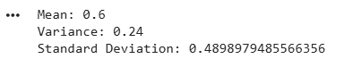
Output
Step5: Plot the Bernoulli Distribution
- **plt.bar(x, pmf_values) : Creates a bar chart for the two possible outcomes (0 and 1).
- **plt.xticks([0, 1]) : Ensures only the valid Bernoulli outcomes appear on the x-axis. Python `
plt.bar(x, pmf_values) plt.xticks([0, 1]) plt.xlabel("X") plt.ylabel("P(X = x)") plt.title("Bernoulli Distribution (p = 0.6)") plt.show()
`
**Output:
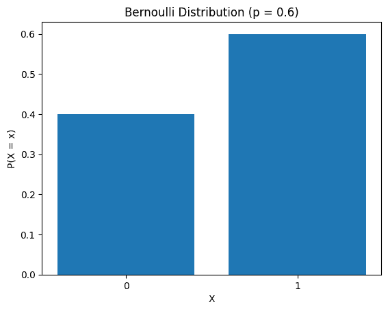
Output
You can download the full code from here
Applications of Bernoulli Distribution in Business Statistics
The Bernoulli Distribution is widely used in business because many real world outcomes are binary (yes/no, success/failure). Some key applications include:
- **Quality Control: Used to check whether a product passes (1) or fails (0) inspection. It helps measure production quality.
- **Market Research: Applied to yes/no survey responses, such as satisfied (1) or not satisfied (0), to understand customer opinions.
- **Risk Assessment: Models outcomes like investment success (1) or failure (0) to evaluate risk levels.
- **Marketing Campaigns: Tracks actions such as email opened (1) or not opened (0) to measure campaign effectiveness.
Bernoulli Distribution vs. Binomial Distribution
The Bernoulli Distribution and the Binomial Distribution are both used to model random experiments with binary outcomes, but they differ in how they handle multiple trials or repetitions of these experiments.
| Bernoulli Distribution | Binomial Distribution | |
|---|---|---|
| **Number of Trials | Single trial | Multiple trials |
| **Possible Outcomes | 2 outcomes (0 or 1) | Multiple outcomes (0, 1, 2, ..., n successes) |
| **Parameter | Probability of success p | Number of trials n and probability p |
| **Random Variable | Indicates success (1) or failure (0) | Counts total number of successes |
| **Purpose | Describes single trial events with success/failure. | Models the number of successes in multiple trials. |
| **Example | Single coin toss, Pass/Fail | Number of heads in 10 tosses, Defective items in a batch |