Lognormal Distribution in Business Statistics (original) (raw)
Last Updated : 23 Jul, 2025
In business statistics, Lognormal Distribution is a crucial probability distribution model as it characterises data with positive values that show right-skewed patterns, which makes it suitable for various real-world scenarios like stock prices, income, resource reserves, social media, etc. Understanding Lognormal Distribution helps in risk assessment, portfolio optimisation, and decision-making in fields, like finance, economics, and resource management.
Table of Content
- Probability Density Function (PDF) of Lognormal Distribution
- Lognormal Distribution Curve
- Mean and Variance of Lognormal Distribution
- Applications of Lognormal Distribution
- Examples of Lognormal Distribution
- Difference Between Normal Distribution and Lognormal Distribution
What is Lognormal Distribution?
The lognormal distribution is a way to describe the likelihood of different values for a variable. This variable has a special property; if logarithm (log) is taken as its value, those log values follow a normal distribution. In layman's language, if we have a variable X that follows a lognormal distribution, then if we take the natural logarithm (ln) of X, we'll get a normal distribution. If X has a lognormal distribution with parameters μ and σ, then, X ~ log N (μ,σ2).
Probability Density Function (PDF) of Lognormal Distribution
The probability density function (PDF) for the lognormal distribution depends on two parameters, μ (mean) and σ (standard deviation), for x values greater than 0. When we take the logarithm of our lognormal data, μ represents the mean, and σ is the standard deviation of this transformed data.
f(x)=\frac{1}{xσ√2π}e^\frac{-1}{2}(\frac{logx-μ}{σ})^2, for ~0<x<\infty
- μ represents the mean or the location parameter.
- σ represents the standard deviation or the shape parameter.
- x is the value for which is required to find the probability density.
- e is mathematical constants.
Lognormal Distribution Curve
- It is right-skewed, meaning it tilts to the right.
- The curve begins at zero, rises to its peak, and then declines.
- The degree of skewness increases as the standard deviation (σ) rises, keeping the mean (μ) constant.
- μ represents the mean of natural logarithms of the data.
- σ represents the standard deviation of natural logarithms of the data.
- When σ is much larger than 1, the curve rises steeply at the start, peaks early, and then falls rapidly, resembling an exponential curve.
- In this distribution, μ acts as more of a scale parameter, unlike the normal distribution where it serves as a location parameter.
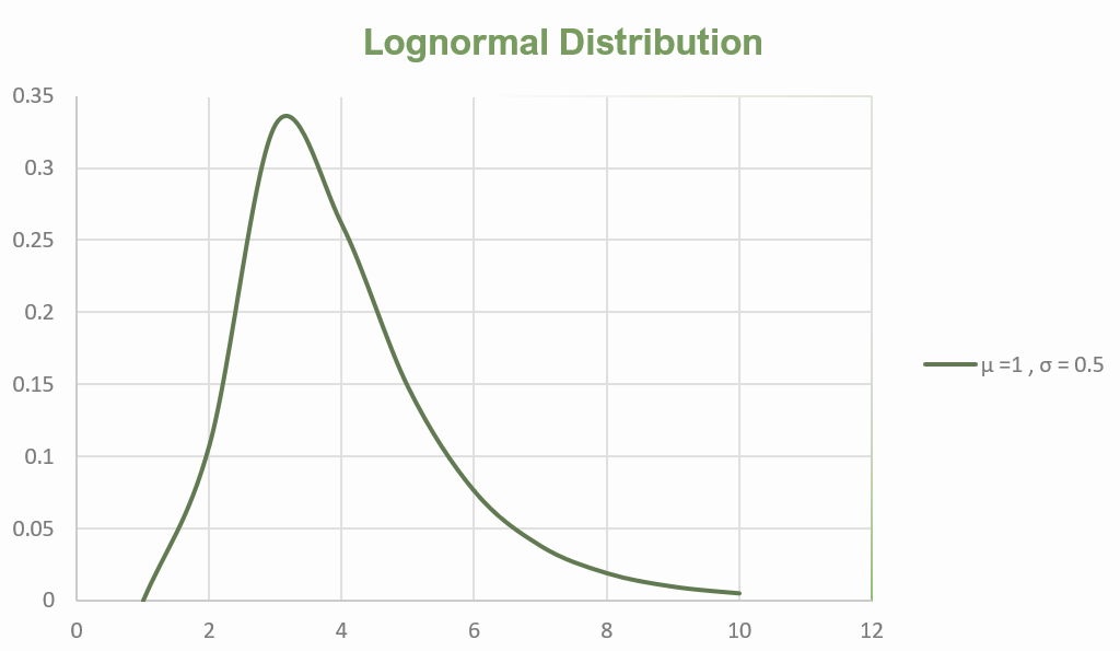
The Probability Density Function (PDF) for the Lognormal Distribution
Mean and Variance of Lognormal Distribution
Mean (μ)
- The mean (μ) of a lognormal distribution is not simply the mean of the original data; it is the mean of the natural logarithm of the data.
- Then, find the mean of these natural logarithms. Mathematically, μ is the average of ln(x), where x represents the original data.
- The mean of the lognormal distribution is not equivalent to the median or the mode of the original data. It is important to remember that the lognormal distribution models the distribution of the logarithms of the data, which can result in quite different characteristics.
μ=e^{μ+{\frac{1}{2}σ^2}}
Where,
- μ represents the mean of the natural logarithm of the data.
- σ represents the standard deviation of the natural logarithm of the data.
- e is the mathematical constant approximately equal to 2.71828.
Variance (σ2)
- The variance (σ2) of a lognormal distribution is similarly calculated from the natural logarithms of the data.
- The standard deviation of the natural logarithm of the data is σ. To get the variance, square this standard deviation that will result in σ2.
- The variance formula involves both σ and μ.
- The variance of the lognormal distribution helps describe how data points are dispersed around the mean of the natural logarithm of the data.
σ^2=(e^{σ^2}-1)e^{2μ+σ^2}
Where,
- The standard deviation of the natural logarithm of the data is represented by σ
- The mean of the natural logarithm of the data is represented by μ
- e is the mathematical constant approximately equal to 2.71828.
Applications of Lognormal Distribution
1. Rubik's Cube Solving Times: The time taken by individuals to solve a Rubik's Cube, whether by an individual or as part of a general population, often follows a lognormal distribution. This distribution can help analyse and predict solving times.
2. Social Media Comments: The length of comments posted on social media discussion forums can be modelled by a lognormal distribution. Understanding the distribution of comment lengths can help in content moderation and engagement analysis.
3. Online Article Reading Time: The time spent by users reading online articles, whether they are news articles, jokes, or other content, can often be described by a lognormal distribution. This information is valuable for content creators and marketers.
4. Income Distribution: In economics, the lognormal distribution is used to analyse income distributions, particularly for the majority of the population and helps in understanding how incomes are spread out among different income groups.
5. Stock Market Fluctuations: Lognormal distributions are used in finance to analyse stock market fluctuations and asset prices. They are particularly useful for modelling the distribution of asset returns, which often exhibit right-skewed patterns.
Examples of Lognormal Distribution
Example 1:
The daily website visitors of a small blog follow a lognormal distribution with a mean of 50 visitors and a geometric standard deviation of 1.1. Calculate the variance of the daily website visitors.
Solution:
To find the variance σ2 we will use the formula for the variance of a lognormal distribution:
σ^2=(e^{σ^2}-1)e^{2μ+σ^2}
Accordng to the given information, we have:
- σ2 is the variance
- μ = 50
- σ = 1.1
putting these values in the formula we get,
σ^2=(e^{1.1^2}-1)·e^{2(50)+1.1^2}
σ^2=(e^{1.21}-1)·e^{(100+1.21)}
σ^2=(3.35-1)\times 9.014
σ2 = 21.1829
∴ Variance of the daily website visitors is approximately 21.1829.
Example 2:
The population of a village follows a lognormal distribution with a median population of 1,000 and a geometric standard deviation of 1.2. Calculate the mean (average) population of the village.
Solution:
To find the mean population μ, you can use the formula for the mean of a lognormal distribution:
μ=e^{μ'}⋅\ e^{\frac{σ^2}{2}}
Accordng to the given information, we have:
- μ is the mean you want to find.
- μ'= ln1000
- σ= 1.2
putting these values in the formula we get,
μ=e^{ln(1000)}⋅\ e^{\frac{1.2^2}{2}}
μ=1000\times{e^{0.72}}
μ = 2051.27
∴ the mean population of the village is approximately 2,051.27.
Difference Between Normal Distribution and Lognormal Distribution
| Characteristic | Normal Distribution | Lognormal Distribution |
|---|---|---|
| Shape | Symmetrical | Right-skewed |
| Range of Values | From negative to positive | From zero to positive |
| Parameter Interpretation | Mean (μ) and Standard Deviation (σ) | Mean of ln(x) (μ) and Standard Deviation of ln(x) (σ) |
| Data Transformation | Not transformed | Natural logarithm transformation of data |
| Applications | Common in many natural phenomena such as heights, weights, IQ scores | Used for data with positive values that exhibit right-skewed patterns, like income, stock prices, and resource reserves |
| Real-life Examples | Heights, weights, IQ scores | Stock returns, resource reserves, income distribution |
| Probability Density Function | Symmetrical bell-shaped curve | Right-skewed, starts from zero and rises to a peak |
| Mean and Variance | Define the central tendency and spread of data | Define the central tendency and spread of the natural logarithm of the data |
| Common Parameter Values | μ (mean) and σ (standard deviation) | μ and σ represent parameters of the natural logarithm of the data |