Normal Distribution (original) (raw)
Last Updated : 27 Dec, 2025
Normal Distribution is the most common or normal form of distribution of Random Variables, hence the name "normal distribution." It is also called the Gaussian Distribution in Statistics or Probability. We use this distribution to represent a large number of random variables. It serves as a foundation for statistics and probability theory.
It also describes many natural phenomena, forms the basis of the Central Limit Theorem, and supports numerous statistical methods.
**Example: Imagine a class where students take a math test. Most students score close to the average mark, and only a few score very low or very high. If we want to describe how these marks are spread around the average in a bell-shaped pattern, this is a situation where we use the normal distribution.
Normal distribution is a continuous probability distribution that is symmetric about the mean, depicting that data near the mean are more frequent in occurrence than data far from the mean.
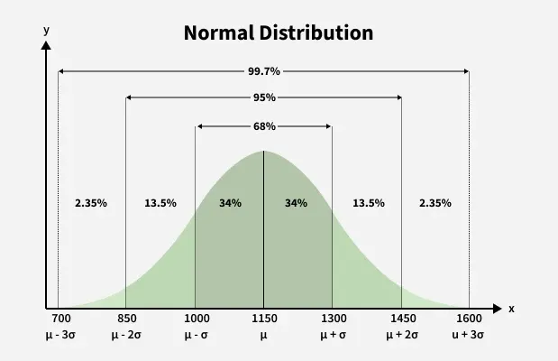
Fig 1: Normal Distribution
As shown in Fig 1, the distribution is symmetric about its center, which is the mean (0 in this case). This symmetry means that events equidistant from the mean have equal probabilities. The density is highest near the mean, resulting in lower probabilities for values farther away from it.
We define Normal Distribution as the probability density function of any continuous random variable for any given system. Now for defining Normal Distribution suppose we take f(x) as the probability density function for any random variable X.
- The area under the curve of a normal distribution is always 1.
- The curve traced by the upper values of the Normal Distribution is in the shape of a Bell, hence Normal Distribution is also called the "**Bell Curve".
Normal Distribution Formula
The formula for the probability density function of the Normal Distribution (Gaussian Distribution) is added below:
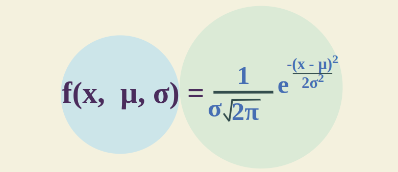
Probability Density Formula for Normal Distribution
where,
- x is Random Variable
- μ is Mean
- σ is Standard Deviation
Normal Distribution Characteristics
- **Symmetry: The normal distribution is symmetric around its mean. This means the left side of the distribution mirrors the right side.
- **Mean, Median, and Mode: In a normal distribution, the mean, median, and mode are all equal and located at the center of the distribution.
- **Bell-shaped Curve: The curve is bell-shaped, indicating that most of the observations cluster around the central peak and the probabilities for values further away from the mean taper off equally in both directions.
- **Standard Deviation: The spread of the distribution is determined by the standard deviation. About 68% of the data falls within one standard deviation of the mean, 95% within two standard deviations, and 99.7% within three standard deviations.
Normal Distribution Examples
We can draw a Normal Distribution for various types of data that include,
- Distribution of Height of People.
- Distribution of Errors in any Measurement.
- Distribution of Blood Pressure of any Patient, etc.
Normal Distribution Curve
In a Normal Distribution, a random variable (_X) is a numerical outcome of a process that follows this distribution. The values of _X are not fixed but instead vary according to the distribution’s properties, where:
- The variable is continuous (can take any real value within a range).
- The distribution is defined by its mean (μ) - the peak of the curve and standard deviation (σ) - which controls the spread of the curve.
The Normal Distribution Curve (also called the Bell Curve or Gaussian Curve) is the graphical representation of this distribution, showing:
- Symmetry around the mean (μ).
- 68-95-99.7% Rule (Empirical Rule) for data spread.
- Asymptotic tails (the curve never touches the x-axis but extends infinitely).
Unlike some distributions, the normal distribution is not strictly "bound" to a finite range—it theoretically spans from −∞ to +∞, though extreme values are highly improbable.
An example of the random variable is, suppose we take a distribution of the height of students in a class, then the random variable can take any value in this case, but is bound by a boundary of 2 ft to 6 ft, as it is generally forced physically.
Standard Deviation of Normal Distribution
The mean of any data spread out as a graph helps us to find the line of symmetry of the graph. Standard Deviation tells us how far the data is spread out from the mean value on either side.
- For smaller values of the standard deviation, the values in the graph come closer and the graph becomes narrower.
- For higher values of the standard deviation, the values in the graph are dispersed more, and the graph becomes wider.
**Empirical Rule of Standard Deviation
Generally, the normal distribution has a positive standard deviation, and the standard deviation divides the area of the normal curve into smaller parts, and each part defines the percentage of data that falls into a specific region. This is called the Empirical Rule of Standard Deviation in Normal Distribution.
**Empirical Rule states that,
- 68% of the data approximately fall within one standard deviation of the mean, i.e. it falls between {**Mean - One Standard Deviation, and Mean + One Standard Deviation}
- 95% of the data approximately fall within two standard deviations of the mean, i.e. it falls between {**Mean - Two Standard Deviation, and Mean + Two Standard Deviation}
- 99.7% of the data approximately fall within a third standard deviation of the mean, i.e. it falls between {**Mean - Third Standard Deviation, and Mean + Third Standard Deviation}

Studying the graph, it is clear that using the Empirical Rule, we distribute data broadly in three parts. Thus, the empirical rule is also called the "68 – 95 – 99.7" rule. The curve is perfectly symmetric around the mean (μ), which is located at the center and marks the highest point of the curve. This mean represents the average value of the datasheet. This distribution is commonly used in real-world statistics to represent things like test scores, height, and measurement errors, where most of the values tend to cluster around the average, and extreme values are less common.
Normal Distribution Table
Normal Distribution Table, which is also called Normal Distribution Z Table, is the table of z-values for normal distribution. This Normal Distribution Z Table is given as follows:
| Z-Value | 0 | 0.01 | 0.02 | 0.03 | 0.04 | 0.05 | 0.06 | 0.07 | 0.08 | 0.09 |
|---|---|---|---|---|---|---|---|---|---|---|
| 0 | 0 | 0.004 | 0.008 | 0.012 | 0.016 | 0.0199 | 0.0239 | 0.0279 | 0.0319 | 0.0359 |
| 0.1 | 0.0398 | 0.0438 | 0.0478 | 0.0517 | 0.0557 | 0.0596 | 0.0636 | 0.0675 | 0.0714 | 0.0753 |
| 0.2 | 0.0793 | 0.0832 | 0.0871 | 0.091 | 0.0948 | 0.0987 | 0.1026 | 0.1064 | 0.1103 | 0.1141 |
| 0.3 | 0.1179 | 0.1217 | 0.1255 | 0.1293 | 0.1331 | 0.1368 | 0.1406 | 0.1443 | 0.148 | 0.1517 |
| 0.4 | 0.1554 | 0.1591 | 0.1628 | 0.1664 | 0.17 | 0.1736 | 0.1772 | 0.1808 | 0.1844 | 0.1879 |
| 0.5 | 0.1915 | 0.195 | 0.1985 | 0.2019 | 0.2054 | 0.2088 | 0.2123 | 0.2157 | 0.219 | 0.2224 |
| 0.6 | 0.2257 | 0.2291 | 0.2324 | 0.2357 | 0.2389 | 0.2422 | 0.2454 | 0.2486 | 0.2517 | 0.2549 |
| 0.7 | 0.258 | 0.2611 | 0.2642 | 0.2673 | 0.2704 | 0.2734 | 0.2764 | 0.2794 | 0.2823 | 0.2852 |
| 0.8 | 0.2881 | 0.291 | 0.2939 | 0.2967 | 0.2995 | 0.3023 | 0.3051 | 0.3078 | 0.3106 | 0.3133 |
| 0.9 | 0.3159 | 0.3186 | 0.3212 | 0.3238 | 0.3264 | 0.3289 | 0.3315 | 0.334 | 0.3365 | 0.3389 |
| 1 | 0.3413 | 0.3438 | 0.3461 | 0.3485 | 0.3508 | 0.3531 | 0.3554 | 0.3577 | 0.3599 | 0.3621 |
| 1.1 | 0.3643 | 0.3665 | 0.3686 | 0.3708 | 0.3729 | 0.3749 | 0.377 | 0.379 | 0.381 | 0.383 |
| 1.2 | 0.3849 | 0.3869 | 0.3888 | 0.3907 | 0.3925 | 0.3944 | 0.3962 | 0.398 | 0.3997 | 0.4015 |
| 1.3 | 0.4032 | 0.4049 | 0.4066 | 0.4082 | 0.4099 | 0.4115 | 0.4131 | 0.4147 | 0.4162 | 0.4177 |
| 1.4 | 0.4192 | 0.4207 | 0.4222 | 0.4236 | 0.4251 | 0.4265 | 0.4279 | 0.4292 | 0.4306 | 0.4319 |
| 1.5 | 0.4332 | 0.4345 | 0.4357 | 0.437 | 0.4382 | 0.4394 | 0.4406 | 0.4418 | 0.4429 | 0.4441 |
| 1.6 | 0.4452 | 0.4463 | 0.4474 | 0.4484 | 0.4495 | 0.4505 | 0.4515 | 0.4525 | 0.4535 | 0.4545 |
| 1.7 | 0.4554 | 0.4564 | 0.4573 | 0.4582 | 0.4591 | 0.4599 | 0.4608 | 0.4616 | 0.4625 | 0.4633 |
| 1.8 | 0.4641 | 0.4649 | 0.4656 | 0.4664 | 0.4671 | 0.4678 | 0.4686 | 0.4693 | 0.4699 | 0.4706 |
| 1.9 | 0.4713 | 0.4719 | 0.4726 | 0.4732 | 0.4738 | 0.4744 | 0.475 | 0.4756 | 0.4761 | 0.4767 |
| 2 | 0.4772 | 0.4778 | 0.4783 | 0.4788 | 0.4793 | 0.4798 | 0.4803 | 0.4808 | 0.4812 | 0.4817 |
Applications of Normal Distribution in Computer Science
**Feature Scaling (Standardization) in Machine Learning
- Data is transformed to have μ = 0, σ = 1 (Z-score normalization).
- Improves the performance of algorithms like SVM, KNN, and Neural Networks.
**Bayesian Inference & Probabilistic Models
- Assumes Gaussian priors in Bayesian networks.
- Used in Gaussian Mixture Models (GMM) for clustering.
**Anomaly Detection
- Outliers are detected if they fall beyond μ ± 3σ.
- Used in fraud detection, network security.
**Gaussian Blurring
- Applies a normal-distributed kernel to smooth images.
- Reduces noise while preserving edges.
**Diffusion Models (Generative AI)
- Noise is added/removed in a Gaussian process (e.g., Stable Diffusion).
Solved Examples of Normal Distribution
Let's solve some problems with Normal Distribution.
**Example 1: Find the probability density function of the normal distribution of the following data. x = 2, μ = 3 and σ = 4.
**Solution:
Given,
- Variable (x) = 2
- Mean = 3
- Standard Deviation = 4
Using formula of probability density of normal distribution
f(x,\mu , \sigma ) =\frac{1}{\sigma \sqrt{2\pi }}e^\frac{-(x-\mu)^2}{2\sigma^{2}}
Simplifying,
f(2, 3, 4) = 0.09666703
**Example 2: If the value of the random variable is 4, the mean is 4, and the standard deviation is 3, then find the probability density function of the Gaussian distribution.
**Solution:
Given,
- Variable (x) = 4
- Mean = 4
- Standard Deviation = 3
Using formula of probability density of normal distribution
f(x,\mu , \sigma ) =\frac{1}{\sigma \sqrt{2\pi }}e^\frac{-(x-\mu)^2}{2\sigma^{2}}
Simplifying,
f(4, 4, 3) = 1/(3√2π)e0
f(4, 4, 3) = 0.13301
Related Articles
Practice Problems on Normal Distribution
**Question 1: A normal distribution has a mean of 50 and a standard deviation of 5. What is the probability that a randomly selected value from this distribution is less than 45?
**Question 2: If a dataset follows a normal distribution with a mean of 100 and a standard deviation of 15, what is the Z-score for a value of 130? Interpret the Z-score.
Question 3: Given a normal distribution with a mean of 70 and a standard deviation of 10, find the probability that a randomly selected value falls between 60 and 80.
**Question 4: In a normally distributed dataset with a mean of 80 and a standard deviation of 10, what value corresponds to the 90th percentile?
**Question 5: A sample of 30 students has an average test score of 78 with a standard deviation of 12. Assuming the distribution of test scores is normal, what is the probability that the sample mean score is greater than 82?