Solving Linear Equations Data Science (original) (raw)
Last Updated : 20 Mar, 2026
Linear Algebra is important in Data Science as it helps represent and process data efficiently, especially for high-dimensional datasets. It also helps in understanding relationships between variables. This is useful in the following ways:
- **Efficient Data Representation: Organizes data in matrix form
- **Find Relationships: Identifies important variables and patterns
- **Supports ML Algorithms: Forms the basis of many machine learning methods
Detecting Linear Relationships Between Attributes
Linear relationships among attributes are identified using the concepts of null space and nullity. These concepts help determine whether variables are linearly dependent and whether some attributes can be expressed as combinations of others.
A generalized system of linear equations is represented as:
A x = b
**Where:
- A is an m x n matrix of coefficients
- x is an n x 1 vector of unknown variables
- b is an m x 1 dependent variable vector
- m represents the number of equations
- n represents the number of variables
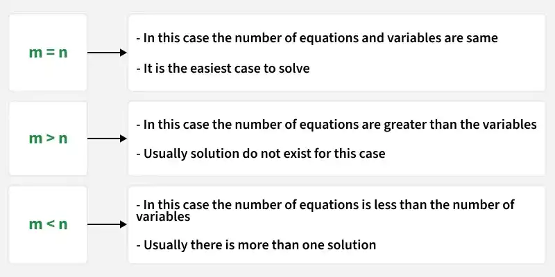
m vs n Cases
Rank Conditions in Linear Systems
In general there are three cases that need to be understood when analyzing linear systems. These cases depend on the rank of the matrix and describe how rows and columns relate to one another. Each case is considered independently.
Case 1: m = n
The solution for this type of linear equation if A is a full rank matrix having determinant of A is equal to 0 will be:
Ax=b
x=A^{-1}b
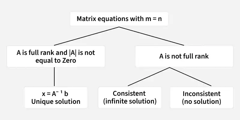
Matrix Solution Cases
**1. Unique Solution
Consider the given matrix equation
\begin{bmatrix} 1 & 3 \\ 2 & 4 \end{bmatrix} \begin{bmatrix} x_1 \\ x_2 \end{bmatrix} = \begin{bmatrix} 7 \\ 10 \end{bmatrix}
- |A| is not equal to zero
- rank(A) = 2: no. of columns this implies that A is full rank
x = \begin{bmatrix} 1 & 3 \\ 2 & 4 \end{bmatrix}^{-1} \begin{bmatrix} 7 \\ 10 \end{bmatrix} = \begin{bmatrix} 1 \\ 2 \end{bmatrix}
Therefore, the solution for the given example is (x1 , x2) = (1, 2)
**2. Infinite Solutions
Consider the given matrix equation
\begin{bmatrix} 1 & 2 \\ 2 & 4 \end{bmatrix} \begin{bmatrix} x_1 \\ x_2 \end{bmatrix} = \begin{bmatrix} 5 \\ 10 \end{bmatrix}
- |A| is not equal to zero
- rank(A) = 1, nullity = 1
Checking consistency
\begin{bmatrix} x_{1} & 2x_{2} \\ 2x_{1} & 4x_{2} \end{bmatrix} = \begin{bmatrix} 5 \\ 10 \end{bmatrix}
Row 2 is twice Row 1 so the system has only one linearly independent equation. Since there are two variables but only one independent equation, the system is consistent and has infinitely many solutions.
- The system has only one linearly independent equation
x_{1}+2x_{2}=5
- We can choose any value for x2. For each choice of x2, there is a corresponding x2.
- Therefore, there are infinitely many solutions to the system.
**3. No Solution
Consider the given matrix equation:
\begin{bmatrix} 1 & 2 \\ 2 & 4 \end{bmatrix} \begin{bmatrix} x_1 \\ x_2 \end{bmatrix} = \begin{bmatrix} 5 \\ 9 \end{bmatrix}
- |A| is not equal to zero
- rank(A) = 1
- nullity = 1
Checking consistency
\begin{bmatrix} x_1 & 2x_2 \\ 2x_1 & 42x_2 \end{bmatrix} = \begin{bmatrix} 5 \\ 9 \end{bmatrix}
Compare Row 2 with 2 × Row 1:
2(x_{1}+2x_{2})=2x_{1}+4x_{2}=10\neq9
We cannot find the solution to (x1, x2)
**Case 2: m > n
- In this case the number of variables or attributes is less than the number of equations.
- Here not all the equations can be satisfied.
- So it is sometimes termed as a case of no solution.
- But we can try to identify an appropriate solution by viewing this case from an optimization perspective.
**An optimization perspective
Instead of finding an exact solution to the system A x = b, we can find an x that minimizes the difference Ax-b.
Let the error vector be:
e=Ax-b
We can minimize all the errors collectively by minimizing \sum_{i=1}^{m} e_i^{2}
So, the optimization problem becomes
\begin{aligned} \sum_{i=1}^{m} e_i^{2}&=min[(Ax-b)^{T}(Ax-b)] \\&=min[(x^{T}A^{T}-b^{T})(Ax-b)]\\&=f(x) \end{aligned}
Here, we can notice that the optimization problem is a function of _x. When we solve this optimization problem, it will give us the solution for _x. We can obtain the solution to this optimization problem by differentiating f(x)with respect to _x and setting the differential to zero.
\nabla f(x)=0
Now, differentiating f(x) and setting the differential to zero results in
\begin{aligned} \nabla f(x) &= 0 \\ 2(A^{T}A)x - 2A^{T}b &= 0 \end{aligned}
Assuming that all the columns are linearly independent
x = (A^{T}A)^{-1}A^{T}b
**Note: While this solution x might not satisfy all the equations but it will ensure that the errors in the equations are collectively minimized.
**Example
Consider the given matrix equation:
\begin{bmatrix} 1&0\\ 2&0\\ 3&1\\ \end{bmatrix} % \begin{bmatrix} x_1\\ x_2\\ \end{bmatrix} = \begin{bmatrix} 1\\ -0.5\\ 5\\ \end{bmatrix}
Here m=3, n=2
Using the optimization concept
\begin{aligned} x &= (A^{T}A)^{-1}A^{T}b \\\begin{bmatrix} x_1\\ x_2\\ \end{bmatrix} &= \begin{bmatrix} 0.2&-0.6\\ -0.6&2.8\\ \end{bmatrix} \begin{bmatrix} 15\\ 5\\ \end{bmatrix} \\ &= \begin{bmatrix} 0\\ 5\\ \end{bmatrix} \end{aligned}
Therefore, the solution for the given linear equation is (x_1, x_2) = (0, 5)
Substituting in the equation shows
\begin{bmatrix} 1&0\\ 2&0\\ 3&1\\ \end{bmatrix} % \begin{bmatrix} 0\\ 5\\ \end{bmatrix} = \begin{bmatrix} 0\\ 0\\ 5\\ \end{bmatrix} \neq \begin{bmatrix} 1\\ -0.5\\ 5\\ \end{bmatrix}
So the important point to notice in case 2 is that if we have more equations than variables then we can always use the least square solution which is x = (A^{T}A)^{-1}A^{T}b .
There is one thing to keep in mind is that (A^{T}A)^{-1} exists if the columns of A are linearly independent.
**Case 3: m < n
- This case deals with more number of attributes or variables than equations
- Here we can obtain multiple solutions for the attributes
- This is an infinite solution case.
- We will see how we can choose one solution from the set of infinite possible solution
Given below is the optimization problem min\left[ \frac{1}{2}x^{T}x \right]such that, Ax=b
We can define a Lagrangian function
min[ f(x, \lambda)] =min\left[ \frac{1}{2}x^{T}x + \lambda^{T}(Ax-b) \right]
Differentiate the Lagrangian with respect to x and set it to zero, then we will get,
\begin{aligned} x + A^{T}\lambda &= 0 \\ x &= -A^{T}\lambda \end{aligned}
Pre - multiplying by A
\begin{aligned} Ax&=b \\A(-A^{T}\lambda) &= b \\ \end{aligned}
assuming that all the rows are linearly independent
\begin{aligned} x &= -A^{T}\lambda \\ &= A^{T}(AA^{T})^{-1}b \end{aligned}
**Example
Consider the given matrix equation:
\begin{bmatrix} 1&2&3\\ 0&0&1\\ \end{bmatrix} % \begin{bmatrix} x_1\\ x_2\\ x_3\\ \end{bmatrix} = \begin{bmatrix} 2\\ 1\\ \end{bmatrix}
Here m=2 and n=3
Using the optimization concept
\begin{aligned} x &= A^{T}(AA^{T})^{-1}b \\ &= \begin{bmatrix} 1&0\\ 2&0\\ 3&1\\ \end{bmatrix} \left( \begin{bmatrix} 1&2&3\\ 0&0&1\\ \end{bmatrix} \begin{bmatrix} 1&0\\ 2&0\\ 3&1\\ \end{bmatrix} \right )^{-1} \begin{bmatrix} 2\\ 1\\ \end{bmatrix} \\ &= \begin{bmatrix} 1&0\\ 2&0\\ 3&1\\ \end{bmatrix} \begin{bmatrix} -0.2\\ 1.6\\ \end{bmatrix} \\ \begin{bmatrix} x_1\\ x_2\\ x_3\\ \end{bmatrix} &= \begin{bmatrix} -0.2\\ -0.4\\ 1\\ \end{bmatrix} \end{aligned}
The solution for the given sample is (x_1, x_2, x_3 ) = (-0.2, -0.4, 1)
You can easily verify that
\begin{bmatrix} 1&2&3\\ 0&0&1\\ \end{bmatrix} \begin{bmatrix} x_1\\ x_2\\ x_3\\ \end{bmatrix} = \begin{bmatrix} 2\\ 1\\ \end{bmatrix}
**Generalization
- The above-described cases cover all the possible scenarios that one may encounter while solving linear equations.
- The concept we use to generalize the solutions for all the above cases is called Moore - Penrose Pseudoinverse of a matrix.
- Singular Value Decomposition can be used to calculate the psuedoinverse or the generalized inverse (A^+).
Properties of Matrix Rank
The row rank of a matrix is always equal to its column rank, regardless of the matrix size
- This means the number of linearly independent rows is equal to the number of linearly independent columns
- For a matrix of size m x n the maximum possible rank is the minimum of m and n, denoted as min (m, n)
- For a matrix of size m x n the maximum possible rank is min(m,n)
- If m < n, the rank of the matrix cannot exceed mmm similarly, if n < m, the rank cannot exceed n
Full Row Rank vs Full Column Rank
Consider a matrix A of size m x n
Full Row Rank
- A matrix has full row rank if all its rows are linearly independent
- No row can be written as a linear combination of other rows
- Each row contributes unique information to the matrix
- The rank of the matrix is equal to the number of rows (m)
- Indicates that data samples are independent and do not show linear dependence
Full Column Rank
- A matrix has full column rank if all its columns are linearly independent
- No column can be written as a linear combination of other columns
- Each column contributes unique information to the matrix
- The rank of the matrix is equal to the number of columns (n)
- Indicates that attributes (features) are linearly independent