Gradient Boosting in R (original) (raw)

Last Updated : 23 Jul, 2025

In this article, we will explore how to implement Gradient Boosting in R, its theory, and practical examples using various R packages, primarily gbm and xgboost.

Gradient Boosting in R

Gradient Boosting is a powerful machine-learning technique for regression and classification problems. It builds models sequentially by combining the outputs of several weak learners (typically decision trees) to form a strong predictive model. In each iteration, it improves the model by minimizing the error of the previous predictions. The **boosting mechanism in gradient boosting optimizes the model to focus on instances where previous predictions were incorrect. Key Concepts of this:

• **Boosting: Boosting is an ensemble learning method that combines multiple weak models (often decision trees) to improve predictive accuracy.
• **Gradient Boosting: Gradient Boosting iteratively trains new models to correct the errors of the prior models. It focuses on minimizing the loss function using gradient descent.
• **Weak Learners: These are simple models, usually decision trees with shallow depth (often called stumps), that individually may not perform well but when combined, produce a strong model.
• **Learning Rate: This controls the contribution of each weak learner to the final model. A smaller learning rate requires more iterations but usually improves performance.
• **Number of Trees: Represents the number of boosting rounds (iterations). More trees can improve the model but also increase the risk of overfitting.
• **Max Depth: Limits the depth of each tree. Smaller depth limits the complexity of individual trees.

Gradient Boosting with the gbm Package

The gbm package provides an efficient way to implement Gradient Boosting in R. It allows you to control various hyperparameters such as the number of trees, depth of trees, learning rate, and more.

Step 1: Load Libraries and Data

We will use the Boston dataset from the MASS package to predict house prices based on several features:

R `

Load necessary libraries

library(gbm) library(MASS)

Load the Boston housing dataset

data(Boston) head(Boston)

`

**Output:

 crim zn indus chas   nox    rm  age    dis rad tax ptratio  black lstat medv  

1 0.00632 18 2.31 0 0.538 6.575 65.2 4.0900 1 296 15.3 396.90 4.98 24.0
2 0.02731 0 7.07 0 0.469 6.421 78.9 4.9671 2 242 17.8 396.90 9.14 21.6
3 0.02729 0 7.07 0 0.469 7.185 61.1 4.9671 2 242 17.8 392.83 4.03 34.7
4 0.03237 0 2.18 0 0.458 6.998 45.8 6.0622 3 222 18.7 394.63 2.94 33.4
5 0.06905 0 2.18 0 0.458 7.147 54.2 6.0622 3 222 18.7 396.90 5.33 36.2
6 0.02985 0 2.18 0 0.458 6.430 58.7 6.0622 3 222 18.7 394.12 5.21 28.7

The Boston dataset contains 506 rows and 14 columns, with the target variable medv representing the median house value.

Step 2: Split the Data into Training and Test Sets

We will split the data into training and test sets to evaluate the performance of the model.

R `

set.seed(123) train_index <- sample(1:nrow(Boston), 0.7 * nrow(Boston)) train_data <- Boston[train_index, ] test_data <- Boston[-train_index, ]

`

Step 3: Fit a Gradient Boosting Model

Now, we will train a Gradient Boosting model using the gbm() function. In this example, we are predicting the medv (median house value) using the remaining variables.

R `

Train the Gradient Boosting model

gbm_model <- gbm( formula = medv ~ ., data = train_data, distribution = "gaussian", n.trees = 5000, interaction.depth = 4, shrinkage = 0.01, cv.folds = 5 )

`

• distribution : This specifies the loss function. For regression, use "gaussian"; for classification, use "bernoulli."
• n.trees : Number of trees (boosting iterations).
• interaction.depth : Depth of individual trees.
• shrinkage : Learning rate (small values slow down the learning process, making it more accurate).
• cv.folds : Cross-validation folds to avoid overfitting.

Step 4: Evaluate the Model

After training the model, we can evaluate its performance on the test dataset. We use the model to predict the medv values for the test dataset and calculate the root mean squared error (RMSE) for performance evaluation.

R `

Make predictions

predictions <- predict(gbm_model, newdata = test_data, n.trees = gbm_model$n.trees)

Calculate RMSE

rmse <- sqrt(mean((predictions - test_data$medv)^2)) print(paste("RMSE:", round(rmse, 2)))

`

**Output:

[1] "RMSE: 3.3"

Step 5: Visualize the Results

We can plot the relative importance of each feature in the model:

R `

Plot feature importance

summary(gbm_model)

`

**Output:

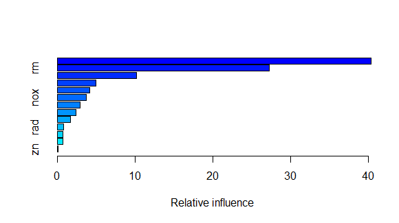
Visualize the Results

This will give a bar plot showing which variables contributed most to the model’s predictions.

Gradient Boosting with the xgboost Package

The xgboost package is another highly efficient and widely used library for implementing gradient boosting in R. It is known for its speed and performance.

Step 1: Data Preparation

xgboost requires the data to be in matrix form. We will prepare the data accordingly:

R `

library(xgboost)

Prepare data matrices

train_matrix <- as.matrix(train_data[,-14]) test_matrix <- as.matrix(test_data[,-14]) train_label <- train_data$medv test_label <- test_data$medv

`

Step 2: Train the XGBoost Model

We can train the model using the xgboost() function:

R `

Train the XGBoost model

xgb_model <- xgboost( data = train_matrix, label = train_label, nrounds = 100, max_depth = 4, eta = 0.1, objective = "reg:squarederror", verbose = 0 )

`

• nrounds : Number of boosting rounds (trees).
• max_depth : Maximum depth of trees.
• eta : Learning rate (similar to shrinkage in gbm).
• objective : Loss function, where "reg" is used for regression.

Step 3: Evaluate the Model

We can now evaluate the model using the test data and calculate the RMSE.

R `

Make predictions

xgb_predictions <- predict(xgb_model, test_matrix)

Calculate RMSE

xgb_rmse <- sqrt(mean((xgb_predictions - test_label)^2)) print(paste("RMSE (XGBoost):", round(xgb_rmse, 2)))

`

**Output:

[1] "RMSE (XGBoost): 3.59"

Step 4: Feature Importance

We can plot the feature importance using xgb.plot.importance():

R `

Plot feature importance

importance <- xgb.importance(feature_names = colnames(train_matrix), model = xgb_model) xgb.plot.importance(importance_matrix = importance)

`

**Output:

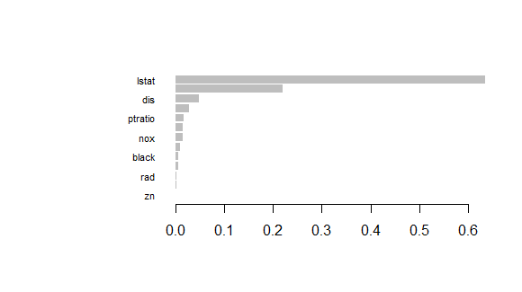
Gradient Boosting in R

This will display the importance of each feature in the XGBoost model.

Tuning Gradient Boosting Models

Both gbm and xgboost allow extensive hyperparameter tuning. Important parameters to tune include:

1. **Learning rate: A smaller learning rate (shrinkage or eta) often leads to better performance but requires more boosting rounds.
2. **Max depth: Controls the complexity of individual trees.
3. **Number of trees: Too many trees can lead to overfitting, while too few may underfit.
4. **Cross-validation: Use cross-validation to avoid overfitting and ensure better generalization.

Conclusion

Gradient Boosting is a powerful and flexible machine learning technique that builds models sequentially to minimize prediction errors. In R, the gbm and xgboost packages provide easy-to-use implementations of Gradient Boosting, enabling you to build strong predictive models for both regression and classification tasks.

• Gradient Boosting combines weak learners (decision trees) to form a strong model.
• The gbm and xgboost packages in R allow efficient Gradient Boosting model building.
• Important parameters such as learning rate, max depth, and number of trees need to be tuned for optimal model performance.
• Cross-validation is crucial to avoid overfitting.

By understanding and applying Gradient Boosting in R, you can greatly enhance your predictive modeling capabilities across various domains.