Skin Cancer Detection using TensorFlow (original) (raw)

Last Updated : 23 Jan, 2026

We will learn how to implement a Skin Cancer Detection model using Tensorflow. We will use a dataset that contains images for the two categories that are malignant or benign. We will use the transfer learning technique to achieve better results in less amount of training.

1. Importing Libraries

**Python libraries make it very easy for us to handle the data and perform typical and complex tasks with a single line of code.

**Pandas: This library helps to load the data frame in a 2D array format and has multiple functions to perform analysis tasks in one go.
**Numpy: Numpy arrays are very fast and can perform large computations in a very short time.
**Matplotlib: This library is used to draw visualizations.
**Sklearn: This module contains multiple libraries having pre-implemented functions to perform tasks from data preprocessing to model development and evaluation.
**Tensorflow: This is an open-source library that is used for Machine Learning and Artificial intelligence and provides a range of functions to achieve complex functionalities with single lines of code. Python `

import numpy as np import pandas as pd import seaborn as sb import matplotlib.pyplot as plt

from glob import glob from PIL import Image from sklearn.model_selection import train_test_split

import tensorflow as tf from tensorflow import keras from keras import layers from functools import partial

AUTO = tf.data.experimental.AUTOTUNE import warnings warnings.filterwarnings('ignore')

2. Load Image Paths

Fetches all image file paths recursively from the dataset directory using glob or you can download dataset from kaggle.

Python `

images = glob('train_cancer//.jpg') len(images)

**Output:

2637

3. Create DataFrame

Standardizes file paths and creates a DataFrame mapping each image path to its label based on the directory.

Python `

#replace backslash with forward slash to avoid unexpected errors images = [path.replace('\', '/') for path in images] df = pd.DataFrame({'filepath': images}) df['label'] = df['filepath'].str.split('/', expand=True)[1] df.head()

**Output:

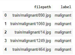
Output

Converting string labels into binary values (0 for benign, 1 for malignant) will save our work of label encoding.

Python `

df['label_bin'] = np.where(df['label'].values == 'malignant', 1, 0) df.head()

**Output:

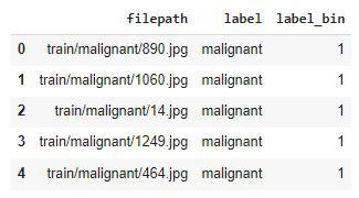
Output

4. Label Distribution

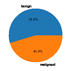
Visualizes the proportion of benign vs malignant images using a pie chart.

Python `

x = df['label'].value_counts() plt.pie(x.values, labels=x.index, autopct='%1.1f%%') plt.show()

**Output:

Output

An approximately equal number of images have been given for each of the classes so, data imbalance is not a problem here.

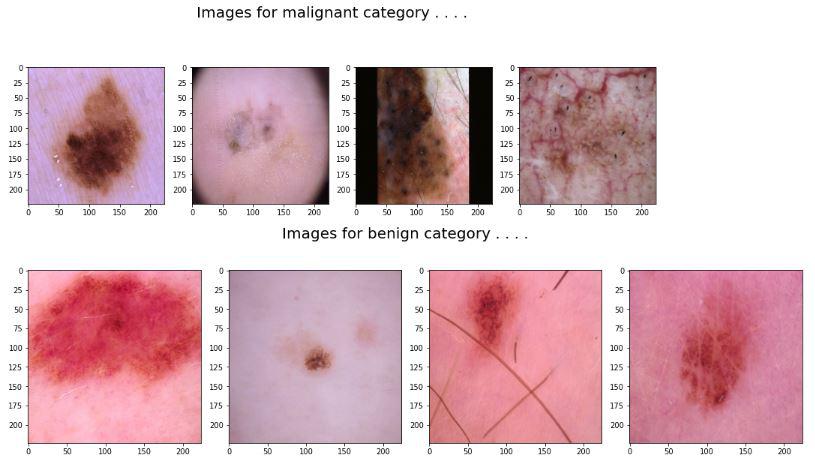
**5. Preview Images

Displays a few sample images from each class for initial visual inspection.

Python `

for cat in df['label'].unique(): temp = df[df['label'] == cat]

index_list = temp.index
fig, ax = plt.subplots(1, 4, figsize=(15, 5))
fig.suptitle(f'Images for {cat} category . . . .', fontsize=20)
for i in range(4):
    index = np.random.randint(0, len(index_list))
    index = index_list[index]
    data = df.iloc[index]

    image_path = data[0]

    img = np.array(Image.open(image_path))
    ax[i].imshow(img)

plt.tight_layout() plt.show()

**Output:

Output

6. Train-Test Split

Now, let's split the data into training and validation parts by using the **train_test_split function.

Python `

features = df['filepath'] target = df['label_bin']

X_train, X_val,
Y_train, Y_val = train_test_split(features, target, test_size=0.15, random_state=10)

X_train.shape, X_val.shape

**Output:

((2241,), (396,))

7. Preprocessing Function

Defines a function to load, decode, resize, and normalize image tensors.

Python `

def decode_image(filepath, label=None):

img = tf.io.read_file(filepath)
img = tf.image.decode_jpeg(img)
img = tf.image.resize(img, [224, 224])
img = tf.cast(img, tf.float32) / 255.0

# Compare label with integer 0 or 1 instead of string
if label == 0: 
    Label = 0
else:
    Label = 1

return img, Label

This code is modified by Susobhan Akhuli

**8. Create Datasets

Image input pipelines have been implemented below so that we can pass them without any need to load all the data beforehand.

Python `

train_ds = ( tf.data.Dataset .from_tensor_slices((X_train, Y_train)) .map(decode_image, num_parallel_calls=AUTO) .batch(32) .prefetch(AUTO) )

val_ds = ( tf.data.Dataset .from_tensor_slices((X_val, Y_val)) .map(decode_image, num_parallel_calls=AUTO) .batch(32) .prefetch(AUTO) )

Now as the data input pipelines are ready let's jump to the modeling part.

9. Model Development

For this task, we will use the EfficientNet architecture and leverage the benefit of pre-trained weights of such large networks.

Model Architecture

We will implement a model using the **Functional API of Keras which will contain the following parts:

The base model is the **EfficientNet model in this case.
The Flatten layer flattens the output of the base model's output.
Then we will have two fully connected layers followed by the output of the flattened layer.
We have included some **BatchNormalization layers to enable stable and fast training and a **Dropout layer before the final layer to avoid any possibility of overfitting.
The final layer is the output layer which outputs soft probabilities for the three classes. Python `

from tensorflow.keras.applications.efficientnet import EfficientNetB7

pre_trained_model = EfficientNetB7( input_shape=(224, 224, 3), weights='imagenet', include_top=False )

for layer in pre_trained_model.layers: layer.trainable = False

**Output:

258076736/258076736 [==============================] - 3s 0us/step

Python `

from tensorflow.keras import Model

inputs = layers.Input(shape=(224, 224, 3)) x = layers.Flatten()(inputs)

x = layers.Dense(256, activation='relu')(x) x = layers.BatchNormalization()(x) x = layers.Dense(256, activation='relu')(x) x = layers.Dropout(0.3)(x) x = layers.BatchNormalization()(x) outputs = layers.Dense(1, activation='sigmoid')(x)

model = Model(inputs, outputs)

10. **Compile Model

While compiling a model we provide these three essential parameters:

**optimizer – This is the method that helps to optimize the cost function by using gradient descent.
**loss – The loss function by which we monitor whether the model is improving with training or not.
**metrics – This helps to evaluate the model by predicting the training and the validation data. Python `

model.compile( loss=tf.keras.losses.BinaryCrossentropy(from_logits=True), optimizer='adam', metrics=['AUC'] )

11. Train Model

Trains the CNN model using the training dataset and validates on the validation set.

Python `

history = model.fit(train_ds, validation_data=val_ds, epochs=5, verbose=1)

**Output:

output

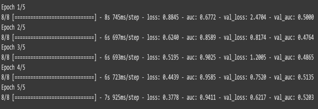
Output

Let’s visualize the training and validation loss and AUC with each epoch.

Python `

hist_df = pd.DataFrame(history.history) hist_df.head()

**Output:

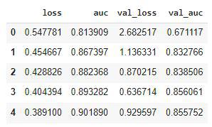
Output

12. Visualization

Python `

hist_df['loss'].plot() hist_df['val_loss'].plot() plt.title('Loss v/s Validation Loss') plt.legend() plt.show()

**Output:

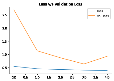
Output

Training loss has not decreased over time as much as the validation loss.

Python `

hist_df['auc'].plot() hist_df['val_auc'].plot() plt.title('AUC v/s Validation AUC') plt.legend() plt.show()

**Output:

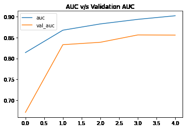
output

Get the Complete Notebook from here.