ML | Common Loss Functions (original) (raw)
Last Updated : 18 Nov, 2025
**Loss functions are a fundamental aspect of **machine learning algorithms, serving as the bridge between **model predictions and the actual outcomes. They quantify how well or poorly a model is performing by calculating the difference between predicted values and actual values. This difference, or "**loss," guides the **optimization process to improve model accuracy. In this article, we will explore various common **loss functions used in **machine learning, categorized into **regression and **classification tasks.
Table of Content
- Importance of Loss Functions in Machine Learning
- Categories of Loss Functions
- Regression Loss Functions in Machine Learning
- Classification Loss Functions in Machine Learning
- Choosing the Right Loss Function
Importance of Loss Functions in Machine Learning
**Loss functions are integral to the training process of **machine learning models. They provide a measure of how well the **model's predictions align with the actual data. By minimizing this **loss, models learn to make more accurate predictions.
The choice of a **loss function can significantly affect the performance of a model, making it crucial to select an appropriate one based on the specific task at hand.
Categories of Loss Functions
The loss function estimates how well a particular algorithm models the provided data. Loss functions are classified into two classes based on the type of learning task
- **Regression Models****:** predict continuous values.
- **Classification Models****:** predict the output from a set of finite categorical values.
By selecting the right **loss function, you optimize the model to meet the task's specific needs, whether it's a **regression or **classification problem.
Regression Loss Functions in Machine Learning
Regression tasks involve predicting continuous values, such as house prices or temperatures. Here are some commonly used loss functions for regression:
**1. **Mean Squared Error (MSE)
It is the Mean of Square of Residuals for all the datapoints in the dataset. Residuals is the difference between the actual and the predicted prediction by the model.
In **machine learning, squaring the residuals is crucial to handle both positive and negative errors effectively. **Since normal errors can be either positive or negative, summing them up might result in a net error of zero, misleading the model to believe it is performing well, even when it is not. To avoid this, we square the residuals, converting all values to positive, which gives a true representation of the model’s performance.
Squaring also has the added benefit of assigning more weight to larger errors, meaning that when the **cost function is far from its minimal value, the model is penalized more heavily for larger mistakes, helping it converge to the minimal value faster.
The **Mean Squared Error (MSE) is a common **loss function in machine learning where the mean of the squared residuals is taken rather than just the sum. This ensures that the **loss function is independent of the number of data points in the training set, making the metric more reliable across datasets of varying sizes. However, **MSE is sensitive to outliers, as large errors have a disproportionately large impact on the final result.
This squaring process is essential for most **regression loss functions, ensuring that models can minimize error and improve performance. The formula is:
MSE = \frac{1}{n} \sum_{i=1}^{n} (y_i - \hat{y}_i)^2
Where:
- yi is the actual value for the i-th data point.
- \hat{y}_i is the predicted value for the i-th data point.
- n is the total number of data points.
**Python implementation:
Python `
import numpy as np
Mean Squared Error
def mse( y, y_pred ) : return np.sum( ( y - y_pred ) ** 2 ) / np.size( y )
`
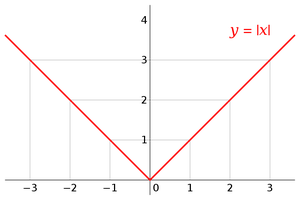
**2. Mean Absolute Error (MAE)
The **Mean Absolute Error (MAE) is a commonly used **loss function in machine learning that calculates the mean of the absolute values of the **residuals for all datapoints in the dataset.
- The absolute value of the residuals is taken to convert any negative differences into positive values, ensuring that all errors are treated equally.
- Taking the mean makes the **loss function independent of the number of datapoints in the training set, allowing it to provide a consistent measure of error across datasets of different sizes.
One key advantage of **MAE is that it is robust to outliers, meaning that extreme values do not disproportionately affect the overall error calculation. However, despite this robustness, **MAE is often less preferred than **Mean Squared Error (MSE) in practice. This is because it is harder to calculate the derivative of the absolute function, as it is not differentiable at the minima. This makes **MSE a more common choice when working with optimization algorithms that rely on gradient-based methods.
This **loss function example illustrates how the choice of a **loss function can significantly impact model performance and training efficiency.
Source: Wikipedia
**The formula:
MAE = \frac{1}{n} \sum_{i=1}^{n} \left| y_i - \hat{y}_i \right|
Where:
- yi is the actual value for the i-th data point.
- \hat{y}_i is the predicted value for the i-th data point.
- n is the total number of data points.
**Python implementation:
Python `
Mean Absolute Error
def mae( y, y_pred ) : return np.sum( np.abs( y - y_pred ) ) / np.size( y )
`
**3. Mean Bias Error
It is similar to **Mean Squared Error (MSE) but provides less accuracy. However, it can help in determining whether the **model has a **positive bias or **negative bias. By analyzing the **loss function results, you can assess whether the model consistently **overestimates or **underestimates the actual values. This insight allows for further refinement of the **machine learning model to improve prediction accuracy. Such **loss function examples are useful in understanding model performance and identifying areas for optimization, making them an essential part of the **machine learning process.
**The formula:
MBE = \frac{1}{n} \sum_{i=1}^{n} \left( y_i - \hat{y}_i \right)
**Python implementation:
Python `
Mean Bias Error
def mbe( y, y_pred ) : return np.sum( y - y_pred ) / np.size( y )
`
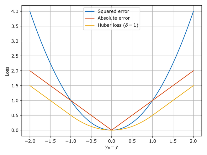
**4. Huber Loss ****/ Smooth Mean Absolute Error**
The **Huber loss function is a combination of **Mean Squared Error (MSE) and **Mean Absolute Error (MAE), designed to take advantage of the best properties of both **loss functions. It is commonly used in **machine learning when training models because it is less sensitive to outliers than **MSE and is still differentiable at its minimum, unlike **MAE.
- When the error is small, the **MSE component of the **Huber loss is applied, making the model more sensitive to small errors.
- Conversely, when the error is large, the **MAE part of the loss function is utilized, reducing the impact of outliers.
A new hyper-parameter, typically called "delta," is introduced to determine the threshold where the **Huber loss switches from **MSE to **MAE. This delta value allows the **loss function to balance the transition between the two. Additional terms involving this hyper-parameter are also incorporated to smooth the shift between **MSE and **MAE, ensuring a seamless transition within the **loss function.
This is a powerful **loss function example that demonstrates the flexibility and effectiveness of **loss functions in machine learning, especially when dealing with datasets containing outliers.
Loss Functions
**The formula:
\text{Loss} = \begin{cases} \frac{1}{2} (x - y)^2 & \text{if } |x - y| \leq \delta \\ \delta \cdot |x - y| - \frac{1}{2} \cdot \delta^2 & \text{otherwise} \end{cases}
Where:
- x is the predicted value.
- y is the actual value.
- \delta is a threshold (hyperparameter) that determines the transition point between the squared error and absolute error.
**Python implementation:
Python `
def Huber(y, y_pred, delta): condition = np.abs(y - y_pred) < delta l = np.where(condition, 0.5 * (y - y_pred) ** 2, delta * (np.abs(y - y_pred) - 0.5 * delta))
return np.sum(l) / np.size(y)`
Classification Loss Functions in Machine Learning
**1. Cross-Entropy Loss
**Cross-Entropy Loss, also known as **Negative Log Likelihood, is a commonly used **loss function in machine learning for **classification tasks. This **loss function measures how well the predicted probabilities match the actual labels.
The **cross-entropy loss increases as the predicted probability diverges from the true label. In simpler terms, the farther the model's prediction is from the actual class, the higher the **loss. This makes **cross-entropy loss an essential tool for improving the accuracy of classification models by minimizing the difference between the predicted and actual labels.
A **loss function example using cross-entropy would involve comparing the predicted probabilities for each class against the actual class label, adjusting the model to reduce this error during training.
**Python implementation:
Python `
Binary Loss
def cross_entropy(y, y_pred): return - np.sum(y * np.log(y_pred) + (1 - y) * np.log(1 - y_pred)) / np.size(y)
`
**The formula:
\text{CrossEntropyLoss} = - \left(y_i \log \left(\hat{y}_i\right) + (1 - y_i) \log \left(1 - \hat{y}_i\right)\right)
**2. Hinge Loss
**Hinge Loss, also known as **Multi-class SVM Loss, is a type of **loss function used for **maximum-margin classification tasks, most commonly applied in **support vector machines (SVMs). This **loss function in machine learning is particularly effective in ensuring that the decision boundary is as far away as possible from any data points. Hinge Loss is a **convex function, making it suitable for optimization using a **convex optimizer.
This type of **loss function is widely used in **classification tasks as it encourages models to achieve a larger margin between different classes, leading to better generalization. A common **loss function example involving Hinge Loss can be seen in SVM models.
**The formula:
\text{SVMLoss} = \sum_{j \neq y_i} \max \left(0, s_j - s_{y_i} + 1 \right)
Where:
- sj is the score (raw output of the classifier, before applying any activation function) for class j.
- syi is the score for the true class label yi .
- The sum is taken over all classes j except the true class label yi .
\begin{equation} \text { SVMLoss }=\sum_{j \neq y_{i}} \max \left(0, s_{j}-s_{y_{i}}+1\right) \end{equation}
**Python implementation:
Python `
Hinge Loss
def hinge(y, y_pred): l = 0 size = np.size(y) for i in range(size): l = l + max(0, 1 - y[i] * y_pred[i]) return l / size
`
3. Kullback-Leibler Divergence (KL Divergence)
**Kullback-Leibler Divergence (KL Divergence) is a widely used **loss function in machine learning that measures how one probability distribution differs from a reference probability distribution. This divergence quantifies the "distance" between the two distributions, making it a crucial tool when comparing them.
In **machine learning, especially in models involving **neural networks, KL Divergence is often applied in tasks where the model outputs are probabilities, such as in **classification tasks using the **softmax function. By minimizing KL Divergence, the model ensures that its predicted probability distribution closely aligns with the true distribution, making it a valuable **loss function example for applications requiring precise probabilistic outputs.
The KL divergence formula:
D_{\text{KL}}(P \parallel Q) = \sum_{i} P(i) \log\left(\frac{P(i)}{Q(i)}\right)
Where:
- DKL(P∥Q) is the Kullback-Leibler divergence between two probability distributions P and Q.
- P(i) is the probability of event iii under distribution P.
- Q(i) is the probability of event iii under distribution Q.
**Python Implementation:
Python `
import numpy as np def kl_divergence(P, Q):#Calculate the Kullback-Leibler (KL) Divergence between two distributions P and Q. # Ensure P and Q are numpy arrays P = np.asarray(P, dtype=np.float32) Q = np.asarray(Q, dtype=np.float32)
# Add a small epsilon to avoid division by zero or log of zero
epsilon = 1e-10
P = np.clip(P, epsilon, 1)
Q = np.clip(Q, epsilon, 1)

return np.sum(P * np.log(P / Q))
`
Choosing the Right Loss Function
The choice of a **loss function in machine learning is influenced by several key factors:
- **Nature of the Task: Determine whether you are dealing with **regression or **classification problems.
- **Presence of **Outliers: Consider how outliers in your dataset may impact your decision; some **loss functions (e.g., **Mean Absolute Error (MAE) and **Huber loss) are more robust to outliers than others.
- **Model Complexity: Simpler models may benefit from more straightforward **loss functions, such as **Mean Squared Error (MSE) or **Cross-Entropy.
- **Interpretability: Some **loss functions provide more intuitive explanations than others, making them easier to understand in practice.