Time Series Modeling with StatsModels (original) (raw)
Last Updated : 23 Jul, 2025
StatsModels is a comprehensive Python library for statistical modeling, offering robust tools for time series analysis. Time Series Analysis module provides a wide range of models, from basic autoregressive processes to advanced state-space frameworks, enabling rigorous analysis of temporal data patterns. The library emphasizes statistical rigor with integrated hypothesis testing and diagnostics.
Key Components of StatsModel 's Time Series Module
Core Models and Functions
- **ARIMA/SARIMAX: For non-seasonal and seasonal integrated autoregressive moving average models.
- **Vector Autoregression (VAR): Models interdependencies in multivariate time series.
- **State Space Models: Flexible framework via SARIMAX, UnobservedComponents, and DynamicFactor.
- **Descriptive Statistics****:** Includes ACF, PACF, periodograms, and stationarity tests (ADF, KPSS).
- **Seasonal Decomposition****:** Separates trend, seasonal, and residual components.
Estimation Methods
- Maximum Likelihood (exact/conditional)
- Kalman Filter-based estimation
- Conditional Least Squares
Step-by-Step Implementation Guide
**Step 1 : Importing Libraries and Preparing the Environment
- pandas and numpy are fundamental for data manipulation.
- matplotlib is used for plotting time series and results.
- SARIMAX from statsmodels is the main modeling class for time series with trend, seasonality, and optional exogenous variables. Python `
import pandas as pd import numpy as np import matplotlib.pyplot as plt from statsmodels.tsa.statespace.sarimax import SARIMAX
`
**Output
Importing Libraries
**Step 2: Loading and Preprocessing and Visualise Data
Python `
Load AirPassengers dataset
url = "https://raw.githubusercontent.com/jbrownlee/Datasets/master/airline-passengers.csv" data = pd.read_csv(url, parse_dates=['Month'], index_col='Month') data = data.rename(columns={'Passengers': 'value'})
Visualize
data.plot(title='Monthly Airline Passengers (1949-1960)') plt.ylabel('Passengers') plt.show()
`
**Output
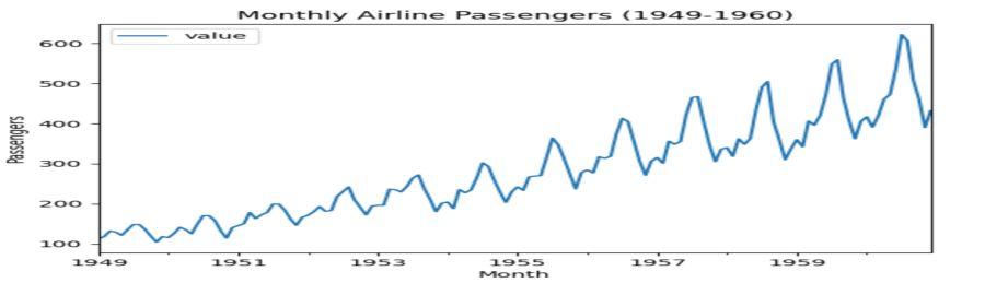
Visualisation
- Loads your time series data from a CSV file.
- Sets the date column as the index and parses it as datetime, which is crucial for time series analysis
- The data is structured so that each row represents a time point (e.g., daily, monthly).
- Ensuring the index is a datetime object allows StatsModels to recognize time ordering and frequencies.
Here, the code:
- **Loads the AirPassengers dataset from a CSV file containing monthly totals of airline passengers from 1949 to 1960, with the "Month" column parsed as a datetime index and the "Passengers" column renamed to "value".
- Plots the time series to visually display how the number of airline passengers changes over time, allowing you to observe overall trends, seasonality, and any anomalies in the data.
**Step 3: Stationarity Check
Python `
Augmented Dickey-Fuller test
adf_result = adfuller(data['value']) print(f'ADF Statistic: {adf_result[0]:.4f}') print(f'p-value: {adf_result[1]:.4f}')
`
**Output
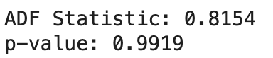
Stationarity Check
It performs the Augmented Dickey-Fuller (ADF) test on your time series data to check if it is stationary. Specifically:
1. The function adfuller(data['value']) tests for the presence of a unit root, which would indicate non-stationarity (i.e., the mean and variance change over time).
2. The output includes an ADF test statistic and a p-value.
- If the **p-value is less than 0.05, you can reject the null hypothesis and conclude the series is stationary.
- If the **p-value is greater than 0.05, you fail to reject the null and the series is likely non-stationary.
**Step 4: Make Data Stationary
Python `
Apply first-order differencing
data_diff = data.diff().dropna() adf_result_diff = adfuller(data_diff['value']) print(f'Differenced ADF Statistic: {adf_result_diff[0]:.4f}') print(f'p-value: {adf_result_diff[1]:.4f}')
`
**Output
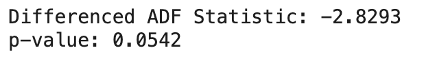
Stationary Data
It applies **first-order differencing to the time series, which means it subtracts each value from its previous value to remove trends and stabilize the mean. Then, it runs the Augmented Dickey-Fuller (ADF) test again on the differenced data to check if the series has become stationary (i.e., its statistical properties no longer depend on time).
**Step 5: Seasonal Decomposition
Python `
decomposition = seasonal_decompose(data, model='multiplicative') decomposition.plot() plt.show()
`
**Output
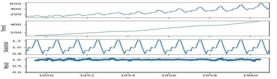
Seasonal Decomposition
This code uses **seasonal decomposition to break down your time series into three separate components: trend (long-term movement), seasonality (regular repeating patterns), and residuals (random noise). The 'multiplicative' model is chosen, meaning the components are multiplied together, which is appropriate when seasonal effects increase or decrease with the trend.
**Step 6: Model Fitting (SARIMAX Example)
Python `
Fit seasonal ARIMA model
model = SARIMAX(data, order=(1,1,1), seasonal_order=(1,1,1,12)) results = model.fit(disp=False)
Summary diagnostics
print(results.summary())
`
**Output
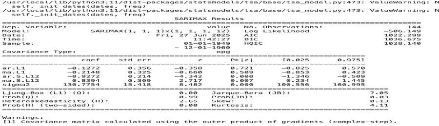
Model Fitting
It fits a **SARIMAX (Seasonal AutoRegressive Integrated Moving Average with eXogenous regressors) model to your time series data, then prints a statistical summary of the results.
- SARIMAX data, order=(1,1,1), seasonal_order=(1,1,1,12)) creates a model that accounts for:
- **Autoregression (AR): Uses past values to predict current values.
- **Integration (I): Applies differencing to make the series stationary.
- **Moving Average (MA): Models the relationship between an observation and past errors.
- **Seasonal components: Captures repeating seasonal patterns (here, yearly seasonality with 12 periods).
- model.fit(disp=False) estimates the model parameters from your data.
- results.summary() displays detailed diagnostics, including estimated coefficients, statistical significance, and model fit metrics.
**Step 7: Forecasting
Python `
Generate 24-month forecast
forecast = results.get_forecast(steps=24) forecast_mean = forecast.predicted_mean conf_int = forecast.conf_int()
Plot results
plt.figure(figsize=(12,6)) plt.plot(data, label='Historical') plt.plot(forecast_mean, color='red', label='Forecast') plt.fill_between(conf_int.index, conf_int.iloc[:,0], conf_int.iloc[:,1], color='pink') plt.title('SARIMAX Forecast with 95% Confidence Interval') plt.legend() plt.show()
`
**Output
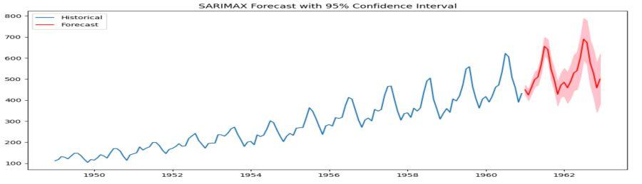
SARIMAX Forecasting
It generates a **24-month forecast using the previously fitted SARIMAX model and visualizes the results:
1. results.get_forecast(steps=24) predicts the next 24 months of values based on the learned patterns in the historical data.
2. forecast.predicted_mean gives the forecasted values, while forecast.conf_int() provides the lower and upper bounds for the 95% confidence interval.
3. The plot displays:
- **Historical data (actual past values)
- **Forecasted future values (in red)
- **Shaded confidence interval (in pink), showing the range where future values are likely to fall
**You can download the complete Source code : Time Series Analysis
Model Types and Applications
| Model Type | Key Features | Best For |
|---|---|---|
| **ARIMA | Autoregressive Integrated Moving Average | Non-seasonal trends |
| **SARIMAX | Seasonal ARIMA with exogenous variables | Complex seasonality |
| **VAR | Vector Autoregression | Multivariate dependencies |
| **State Space | Flexible latent variable modeling | Structural time series |
Considerations
- **Stationarity: Most models require stationary data (constant mean/variance)
- **Model Selection: Use AIC/BIC to compare models (lower values preferred)
- **Residual Diagnostics: Check for autocorrelation (Ljung-Box test) and normality
- **Overfitting: Validate forecasts against holdout datasets