Last Minute Notes Data Structures using C (original) (raw)
Last Updated : 23 Jul, 2025
Data structures are ways to organize and store data so it can be used efficiently. They are essential in computer science for managing and processing information in programs. Common types of data structures include arrays, linked lists, stacks, queues, trees, and graphs. Each structure is designed for specific tasks, such as searching, sorting, or managing hierarchical data. Understanding data structures helps in solving problems faster and writing better algorithms.
Data structures are of two types:
**1. Linear Data Structures: In linear data structures, elements are arranged in a sequential order. Each element is connected to its previous and next element, making traversal straightforward.
**2. Non-Linear Data Structures: In non-linear data structures, elements are not arranged sequentially. They are connected in a hierarchical or network-like structure.
Table of Content
**Arrays
An **array is a data structure used to store multiple elements of the same type in contiguous memory locations. Arrays are simple and widely used for organizing and managing data.
**Declaration:
In C, we can declare an array by specifying its and size or by initializing it or by both.
// Array declaration by specifying size
int arr[10];// Array declaration by initializing elements
int arr[] = {10, 20, 30, 40};// Array declaration by specifying size **and
// initializing elements
int arr[6] = {10, 20, 30, 40}
**Initialization:
int arr[5] = {1, 2, 3, 4, 5};
**Accessing Elements:
arr[0] = 10; // Assigns 10 to the first element
printf("%d", arr[2]); // Prints the third element
Formulas:
Length of Array = UB - LB + 1
Types of Arrays
**1. One-Dimensional Array: Stores elements in a single row.
Example:
int arr[5] = {10, 20, 30, 40, 50};
**2. Multi-Dimensional Array: Represents a matrix or table of data.
Example:
int matrix[2][3] = {
{1, 2, 3},
{4, 5, 6}
};
Given the address of first element, address of any other element is calculated using the formula:-
Loc (arr [k]) = base (arr) + w * k
w = number of bytes per storage location
of for one element
k = index of array whose address we want
to calculate
Elements of two-dimensional arrays (**mXn) are stored in two ways:-
- Column major order: Elements are stored column by column, i.e. all elements of first column are stored, and then all elements of second column stored and so on.
Loc(arr[i][j]) = base(arr) + w (m *j + i)
- Row major order: Elements are stored row by row, i.e. all elements of first row are stored, and then all elements of second row stored and so on.
Loc(arr[i][j]) = base(arr) + w (n*i + j)
Common Operations on Arrays
- **Traversal: Visiting all elements in the array.
for (int i = 0; i < 5; i++) {
printf("%d ", arr[i]);
}
- **Insertion: Adding an element at a specific position.
Requires shifting elements to make space. - **Deletion: Removing an element from a specific position.
Requires shifting elements to fill the gap. - **Searching: Finding an element in the array.
**Linear Search: Sequentially check each element.
Time Complexity:O(n)
**Binary Search: Requires the array to be sorted.
Time Complexity:O(log n) - **Sorting: Arranging elements in ascending or descending order.
Common algorithms: Bubble Sort, Selection Sort, Quick Sort.
read more about - Arrays
**Stacks
A **stack is a linear data structure that follows the **Last In, First Out (LIFO) principle, meaning the element added last is removed first. It is widely used in programming for tasks such as expression evaluation, backtracking, and function call management.
**Basic operations :
**1. Push: Adds an item in the stack. If the stack is full, then it is said to be an Overflow condition. (Top=Top+1). Time Complexity: O(1).
**2. Pop: Removes an item from the stack. The items are popped in the reversed order in which they are pushed. If the stack is empty, then it is said to be an Underflow condition.(Top=Top-1). Time Complexity: O(1).
**3. Peek: Retrieves the top element without removing it. Time Complexity: O(1).
**Infix, prefix, Postfix notations
**Infix notation: X ****+** Y - Operators are written in-between their operands. This is the usual way we write expressions. An expression such as
A * ( B + C ) / D
**Postfix notation (also known as "Reverse Polish notation"): X Y **+ Operators are written after their operands. The infix expression given above is equivalent to
A B C + * D/
**Prefix notation (also known as "Polish notation"): + X YOperators are written before their operands. The expressions given above are equivalent to
/ * A + B C D
Conversion between these notations: Click here
**Implementation of Stack
Stacks can be implemented in C using:
**Tower of Hanoi
It is a mathematical puzzle where we have three rods and n disks. The objective of the puzzle is to move the entire stack to another rod, obeying the following simple rules:
- Only one disk can be moved at a time.
- Each move consists of taking the upper disk from one of the stacks and placing it on top of another stack i.e. a disk can only be moved if it is the uppermost disk on a stack.
- No disk may be placed on top of a smaller disk.
For n disks, total 2n – 1 moves are required
Time complexity : O(2n) [exponential time]
read more about - Stacks
**Queues
A **queue is a linear data structure that follows the **First In, First Out (FIFO) principle. This means the element added first is removed first. Queues are widely used in scenarios like scheduling, buffering, and real-time systems.
**Types of Queues
- **Simple Queue: Follows the standard FIFO principle. Elements are added at the rear and removed from the front.
- **Circular Queue: The last position connects back to the first position, making the queue circular. Efficient use of memory compared to a simple queue.
- **Priority Queue: Each element is associated with a priority, and elements with higher priority are dequeued before others.
- **Deque (Double-Ended Queue): Elements can be added or removed from both ends (front and rear).
Common Operations on Queue
- **Enqueue: Adds an item to the queue. If t he queue is full, then it is said to be an Overflow condition.
- **Dequeue: Removes an item from the queue. The items are popped in the same order in which they are pushed. If the queue is empty, then it is said to be an Underflow condition.
- **Peek:Retrieve the front element without removing it. Time Complexity:
O(1). - **Traversal: Iterating through all elements in the queue. Time Complexity:
O(n).
**Front: Get the front item from queue.
**Rear: Get the last item from queue.
**Implementation of Queue
Queues can be implemented in C using:
read more about - Queues
Linked Lists
A **linked list is a linear data structure where elements (called nodes) are connected using pointers. Unlike arrays, linked lists do not store elements in contiguous memory locations, making them dynamic and flexible for insertion and deletion operations.
Types of Linked Lists
- **Singly Linked List: Each node points to the next node. Traversal is unidirectional. Last node points to
NULL. - **Doubly Linked List: Each node contains two pointers: one to the next node and one to the previous node. Allows bidirectional traversal.
- **Circular Linked List: The last node points back to the first node, forming a circular structure. Can be singly or doubly linked.
- **Doubly Circular Linked List: Combines features of doubly and circular linked lists, where both
nextandpreviouspointers form a circle.
Common Operations on Linked Lists
- **Traversal: Moving through all nodes in the list. Time Complexity:
O(n). - **Insertion: Adding a new node at the beginning, end, or middle. Time Complexity:
O(1)for insertion at the beginning,O(n)for insertion at the end or middle. - **Deletion: Removing a node from the beginning, end, or middle. Time Complexity:
O(1)for deletion at the beginning,O(n)for deletion at the end or middle. - **Search: Finding an element in the linked list. Time Complexity:
O(n).
**Advantages over arrays
- Dynamic Memory Allocation
- Ease of insertion/deletion
- Flexible Size
**Drawbacks
- Random access is not allowed. We have to access elements sequentially starting from the first node. So we cannot do binary search with linked lists.
- Extra memory space for a pointer is required with each element of the list. Representation in C: A linked list is represented by a pointer to the first node of the linked list. The first node is called head. If the linked list is empty, then value of head is NULL.
**Each node in a list consists of at least two parts:
- Data
- Pointer to the next node In C, we can represent a node using structures. Below is an example of a linked list node with an integer data.
// A linked list node
struct node
{
int data;
struct node *next;
};
read more about - Linked List
Tree
A **tree is a non-linear hierarchical data structure consisting of nodes connected by edges. Trees are widely used for organizing data and solving complex computational problems.
Basic Terminology
- **Node: Represents data.
- **Edge: Connection between two nodes.
- **Degree: The number of children a node has.
- **Binary Tree: A tree where each node has at most two children.
- **Path: A sequence of nodes connected by edges.
**Types of Trees
- **General Tree: Nodes can have any number of children.
- **Binary Tree: Each node has at most two children (left and right).
- **Binary Search Tree (BST): A binary tree where the left child contains values less than the parent, and the right child contains values greater than the parent.
- **Balanced Binary Tree: A binary tree where the height difference between the left and right subtrees of any node is at most one. Examples: AVL Tree, Red-Black Tree.
- **Complete Binary Tree: A binary tree where all levels are fully filled except possibly the last, which is filled from left to right.
- **Full Binary Tree: Every node has either 0 or 2 children.
- **Heap: A complete binary tree used for priority queues. Types: Min-Heap, Max-Heap.
- **Trie: A tree used for storing strings or prefixes efficiently.
- **N-ary Tree: A tree where each node can have up to
Nchildren.
Tree Traversal Techniques
Traversal refers to visiting all nodes in a tree. Common techniques are:
**1. Inorder Traversal (Left, Root, Right)
(i) Traverse the left subtree of root in inorder.
(ii) Process the root.
(iii) Traverse the right subtree of root in inorder.
**Example:
void inorder(struct Node* root) {
if (root != NULL) {
inorder(root->left);
printf("%d ", root->data);
inorder(root->right);
}
}
**2. Preorder Traversal (Root, Left, Right)
****(i)** Process the root.
****(ii)** Traverse the left subtree of the root in preorder.
****(iii)** Traverse the right subtree of the root in preorder.
**Example:
void preorder(struct Node* root) {
if (root != NULL) {
printf("%d ", root->data);
preorder(root->left);
preorder(root->right);
}
}
**3.Post-order
(i) Traverse the left subtree of root in post-order.
(ii) Traverse the right subtree of root in post-order.
(iii) Process the root.
**Example:
void postorder(struct Node* root) {
if (root != NULL) {
postorder(root->left);
postorder(root->right);
printf("%d ", root->data);
}
}
**4. Level Order Traversal:
Visits nodes level by level (Breadth-First Search).
**Example: Use a queue to implement this traversal.
Common Operations on Trees
- **Insertion: Add a node to the tree following specific rules (e.g., BST rules).
- **Deletion: Remove a node while maintaining tree properties (e.g., replace with inorder successor in a BST).
- **Search: Find a node in the tree. Time Complexity:
O(log n)in a balanced tree;O(n)in a skewed tree
Binary Search Tree
A **Binary Search Tree (BST) is a special type of binary tree where each node follows the **binary search property:
- The value of the **left child is less than the value of the parent node.
- The value of the **right child is greater than the value of the parent node.
- Inorder traversal of a binary search tree is ascending order of keys in the BST.
Different Operations on Binary Search Tree are:
- Insertion in a BST O (log n) best case, O (n) worst case
- Deletion of leaf node : can be done directly.
- Deletion of node with one child : copy the child to the node and delete the child.
- Deletion of a node with two children : first find the inorder successor of the node, copy the contents of this successor to the node and delete the inorder successor.
read more about - Binary Search Tree
Heap
A **heap is a special tree-based data structure that satisfies the heap property:
- **Max-Heap: The value of each parent node is greater than or equal to the values of its children.
Example:50, 30, 20, 15, 10, 8, 16(root = 50). - **Min-Heap: The value of each parent node is less than or equal to the values of its children.
Example:10, 15, 20, 30, 50, 40(root = 10).
A heap is commonly implemented as a **binary heap, where it is represented as a binary tree.
**Heap Operations
- **Insertion: Add the new element to the end of the heap (last position in the array representation). Restore the heap property by **heapifying up (swap with parent until heap condition is satisfied).
- **Deletion (Removing the Root): Replace the root with the last element in the heap. Restore the heap property by **heapifying down (swap with the larger child in Max-Heap or smaller child in Min-Heap).
- **Heapify: A process of rearranging the elements to maintain the heap property.
- **Heap Sort: A sorting algorithm that builds a heap from an array, repeatedly removes the root, and stores it in sorted order. Time Complexity:
O(n log n).
Heapify Algorithm
Heapify is an algorithm used to convert a binary tree into a **heap. A **heap is a special type of binary tree that satisfies the heap property, which can either be:
- **Max-Heap: The value of each node is greater than or equal to its children.
- **Min-Heap: The value of each node is less than or equal to its children.
How Heapify Works
- Heapify works by making sure that every subtree of a given node follows the heap property.
- The algorithm starts at a node and checks if it satisfies the heap property with respect to its children.
- If a node violates the heap property, it is swapped with the larger (for max-heap) or smaller (for min-heap) of its children, and the process continues recursively.
Example of Heapify (Max-Heap)
- If the root is smaller than one of its children, swap it with the larger child.
- Then, apply the same process recursively for the swapped child until the heap property is restored.
Complexity
- The time complexity of heapify is **O(log n), where nnn is the number of nodes.
read more about - Heap
AVL Tree
An **AVL Tree is a type of self-balancing binary search tree (BST). Named after its inventors, Adelson-Velsky and Landis, it ensures that the height difference (balance factor) between the left and right subtrees of every node is at most 1. This balancing helps maintain efficient operations such as insertion, deletion, and searching
Rotations in AVL Tree
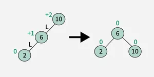
1. Left-Left (LL) Rotation :
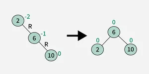
2. Right-Right (RR) Rotation :
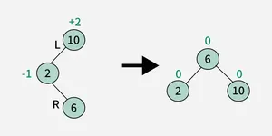
3. Left-Right (LR) Rotation :
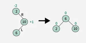
4. Right-Left (RL) Rotation :
Here's a table that outlines various tree operations (like insertion, deletion, etc.) for different types of trees, along with their time complexities:
| **Operation | **Binary Tree | **Binary Search Tree (BST) | **Heap | **AVL Tree |
|---|---|---|---|---|
| **Insertion | O(1) (if position is given) | O(log n) | O(log n) | O(log n) |
| **Deletion | O(1) (if node is given) | O(log n) | O(log n) | O(log n) |
| **Search | O(n) | O(log n) | O(n) (for unsorted) | O(log n) |
| **Traversal | O(n) | O(n) | O(n) | O(n) |
| **Balance Check | O(n) | O(n) | N/A | O(log n) |
| **Height Calculation | O(n) | O(n) | O(n) | O(log n) |
read more about - AVL Tree
Graphs
A **graph is a non-linear data structure consisting of **vertices (nodes) and **edges that connect pairs of vertices. Graphs are widely used to represent relationships between objects in various real-world scenarios like social networks, road maps, and web pages.
Graph Traversal Techniques
**1. Depth First Search (DFS): Traverses as deep as possible along a branch before backtracking. Uses a stack (recursion or explicit).
Example:
C `
void DFS(int vertex, int visited[], int graph[][V]) { printf("%d ", vertex); visited[vertex] = 1; for (int i = 0; i < V; i++) { if (graph[vertex][i] == 1 && !visited[i]) { DFS(i, visited, graph); } } }
`
**2. Breadth First Search (BFS): Traverses all neighbors of a vertex before moving to the next level.
Example:
C `
void BFS(int start, int graph[][V]) { int visited[V] = {0}; int queue[V], front = 0, rear = 0;
queue[rear++] = start;
visited[start] = 1;

while (front != rear) {
    int current = queue[front++];
    printf("%d ", current);

    for (int i = 0; i < V; i++) {
        if (graph[current][i] == 1 && !visited[i]) {
            queue[rear++] = i;
            visited[i] = 1;
        }
    }
}
}
`
read more about - Graphs
Hashing
Hashing is a technique used to map data of arbitrary size to fixed-size values, called hash values or hash codes, using a hash function. It is widely used in computer science for quick data retrieval and efficient storage.
**Hashing Terminology
- **Key: The input value to the hash function.
- **Hash Value: The output of the hash function.
- **Bucket: The location in the hash table where the key-value pair is stored.
- **Load Factor: The ratio of the number of elements to the table size.
Collision Resolution Techniques
**1. Chaining: Uses linked lists to store multiple elements in the same bucket. Each bucket points to a linked list of elements with the same hash value.
**2. Open Addressing: All elements are stored directly in the hash table. On collision, the algorithm probes the table to find an empty slot.
**Probing Techniques:
- **Linear Probing: Search sequentially for the next available slot.
index = (hash + i) % table_size - **Quadratic Probing: Use quadratic intervals to find the next slot.
index = (hash + i^2) % table_size - **Double Hashing: Use a second hash function to find the next slot.
index = (hash1 + i * hash2) % table_size
read more about - Hashing