Basic Elements of Signal Flow Graph (original) (raw)
Last Updated : 9 Mar, 2026
Signal Flow Graphs are a crucial component of control systems. Furthermore, the control system is one of the most significant subjects in Electronics. To understand the Signal Flow Graph, let's understand the Control System first, and then we will dive into the main topic.
- A control system receives an input signal, processes the signal inside an electronic device, and produces an output.
- Signal Flow Graph follows a similar concept where a signal enters at one point and moves through different system elements.
- Mathematical relations and algebraic equations represent signal processing between elements.
- Engineers use this graphical method to easily compute and understand overall system behaviour.
Signal Flow Graph
A **Signal Flow Graph (SFG) is a directed edge and node-based visual depiction of the dynamics of a system. Variables or signals are represented by nodes, while the signal flow between them is shown by edges. SFGs are widely used in control theory because they provide an easy-to-understand representation of intricate system relationships, which helps with analysis and optimization.
Basic Elements of Signal Flow Graph
Nodes and branches are the two basic elements of a Signal Flow Graph.
Node
It is a point that represents a variable or a signal. There are three types of nodes:
- Input Node
- Output Node
- Mixed Node.
To identify a node in a Signal Flow Graph, it is mainly represented with circles or dots; you can find it in the images.
- **Input Node (Source Node): It is a node where we provide only inputs, and it has only outgoing branches. To identify the input node, always follow the arrow. If it enters the node, then it is an input node.
- **Output Node (Sink Node): It is a node that has only incoming branches. To identify the output node, always follow the arrow, if it goes out from node then it is output node.
- **Mixed Node: It is a node that has both incoming and outgoing branches. To identify the mixed node, always follow the arrow, if it has both incoming and outgoing arrow then it is mixed node.
Branch
A branch represents a line segment connecting two nodes in a signal flow graph. Electronic equipment may produce positive or negative gain, and signal movement follows a specific direction. Branch representation therefore includes both gain and direction to complete a signal flow graph. A simple diagram helps in understanding branch connection and signal direction clearly.
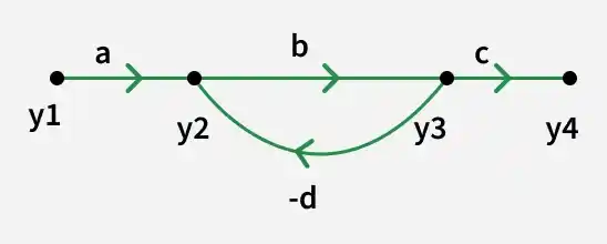
Demo Signal Flow Graph
Here we can see the black dots (y1, y2, y3, y4) they are the nodes of the Signal flow graph, and the lines are the branches. As we see that these branches has some directions that is defined by the arrow symbols. So, we can say a,b,c are the positive gain branches and the d is negative gain branch that is why it is in negative sign.
Characteristics of SFG
- Nodes
- Branches or Edges
- Forward Paths
- Single Loops
- Non-touching Loops
- Mason Gain Formula
How to build Signal Flow Graph?
Let's start building of an new signal flow graph with an algebraic equation, it will help us to understand the complex graphs and how electronics engineers use this in Control System.
**Things to remember: While calculating the result we use the node value (like: y1, y2, y3...) and multiply that with the gain (a, b, c). The value of the node is the resultant value that is obtained by adding both values of a branch to another node.
Here "y1, y2, y3, y4, y5, y6" are the nodes, and "a, b, c, d, e, f, g" are the gains in the Signal Flow Graph respectively.
**Equations:
y2 = ay1, y3 = y2b + y5g, y4 = y3c + y2f, y5 = y4d and y6 = y5e
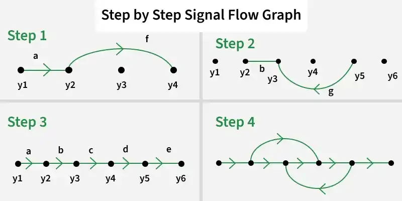
Here we will create the Signal Flow Graph step by step, you can also check the given image below.
- **Step1: Create the first loop, and required branches with the y2 and y4 equation.
- **Step2: Create the second loop, and don't forget the directions with the y3 equation, we have to be careful with the directions. Give directions according to the equations.
- **Step3: Create the main branch with directions, and connect all the nodes with branches.
- **Step4: Now we have to combine the whole structure and we will get the whole Signal Flow Graph, with proper notations and directions.
Signal Flow Graph from Equations
Mason Gain Formula with Example
The Mason's Gain Formula is a mathematical tool used in control system engineering to calculate the overall transfer function of a signal flow graph.
- Nodes, which we already discussed.
- Directed edges, as you can see the above image with the directed arrows.
- Forward paths, which are started and ended on different nodes.
- Loops, which are the close paths in SFG, stared and ended in same node, but passed throw other nodes as well. A SFG can contain many loops.
- Non-touching loops: If there are two or more loops in a single SFG, then they do not touch each other.
**Mason Gain Formula: \frac{C(s)}{R(s)} = \frac{\sum_{i=1}^{N}P_{i}\Delta_{i}}{\Delta}
where,
N: total number of forward paths
Pi : gain of the ith forward path
∆: determinant of the graph
∆i : path-factor for the ith path
The determinant of the graph (∆) and the path-factor for the ith path (∆i) are defined as follows:
∆i : 1 - (loop gain which does not touch the forward path)
∆: 1 - Σ(all individual loop gains) + Σ(gain product of all possible combinations of two non-touching loops) - Σ(gain product of all possible combinations of three non-touching loops) + ....
In this formula the loops of the Signal Flow Graph is very important. In the next example we will see how can we get a transfer function from this formula.
Transfer function T, R is input, C is output, G are the gains and H are the feedbacks of a transfer function.
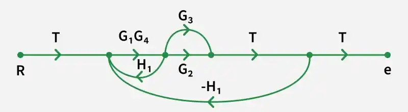
Signal Flow Graph
Here, two paths are available. The transfer function will be:
T=\frac{C(s)}{R(s)} = \frac{P_{1}\Delta_{1}+P_{2}\Delta_{2}}{\Delta}
\frac{C}{R}= \frac{G1G2G4 + G1G3G4}{1-G1G4H1+G1G2G4H2+G1G3G4H2}
**Output: \frac{C(s)}{R(s)} = \frac{G1G4(G2+G3)}{1-G1G4H1+G1G2G4H2+G1G3G4H2}
Signal Flow Graph from Block Diagram
In the field of electronics engineering, block diagrams are used to simplify intricate circuits. The block diagram shows numerous electronic components as well as input and output. As a result, we must carefully comprehend this before drawing the Signal Flow Graph. Prior to that, we must comprehend the jargon.
- R(s) is the input point, C(s) is the output point.
- The circle with a cross is called summing point(S), and the branches meet at the dot point is called take-off point.
- The "**G" inside a box called the gain, there can be many gain blocks in a single block diagram.
- Since electronics components also provide feedback, "H" inside the box is referred to as the feedback.
In the image below we can see the block diagram to Signal Flow Graph:
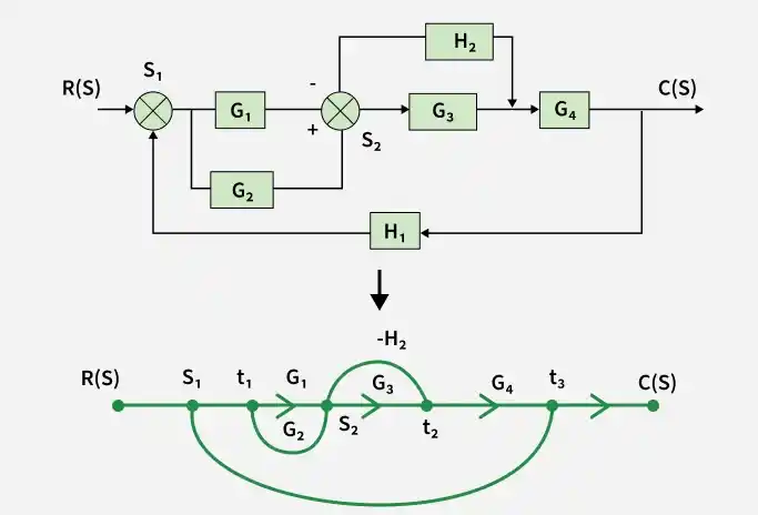
Block Diagram to Signal Flow Graph
R(s) and C(s) is the input and output respectively.
As you can see that in the block diagram there are two summing point so we have mentioned them with S1,S2 in the Signal Flow Graph, and with t1,t2,t3 we mentioned the take-off points.
As, G1 and G2 are in a loop, so we do the same for the Signal Flow Graph also. And feedbacks are in negative so we mentioned it with -H1 and -H2.
So, this is how we made the Signal Flow Graph from Block diagram.
Applications of SFG
- Control System analysis is very much dependent on Signal Flow Graph, because it really helps to calculate and create transfer functions.
- In communication systems, SFGs are employed to model and analyze signal paths, helping engineers to understand the flow of information through a system.
- Signal Flow Graphs are applied to analyze electrical networks, representing voltages and currents.
Advantages and Disadvantages of SFG
Advantages
- A signal flow graph presents a clear view of information flow and system dynamics, which helps engineers understand complex circuits more easily.
- Signal Flow Graphs are useful for examining a system's feedback loops. The influence of feedback on the performance and stability of a system can be recognized and assessed by engineers.
- The transfer function of a system can be systematically derived using the Mason's Gain Formula related to SFGs. This is especially helpful for designing control systems.
Disadvantages
- A signal flow graph provides a clear representation of complex systems. However, very large systems with many interactions may create difficulty because a high number of nodes and branches becomes harder to manage and analyze.
- Signal Flow Graphs are most effective for linear time-invariant (LTI) systems. They may not be as suitable for modeling nonlinear or time-varying systems.
- Signal flow graphs, particularly for systems with delays, may not explicitly reflect causalities in the time domain, despite their ability to depict cause-and-effect linkages.