Excel VLOOKUP Function (original) (raw)
Last Updated : 5 Jun, 2026
VLOOKUP in Excel quickly finds a value in the first column of a table and returns related data from another column. It speeds up data lookup, links information across sheets, and simplifies working with large datasets.
Working of VLOOKUP
VLOOKUP searches vertically down the first column of a table for a specific value and returns a corresponding value from another column.
Common Use Cases
- Finding prices by product ID
- Fetching employee details by ID
- Linking data between sheets or workbooks
Syntax of VLOOKUP
VLOOKUP(lookup_value, table_array, col_index_num, [range_lookup])
- **lookup_value – The value you want to find (ID, name, code, etc.)
- **table_array – The range containing your data
- **col_index_num – Column number (within the table_array) to return data from
- **[range_lookup]_(optional) – Match type
TRUEor omitted → Approximate match (default)FALSE→ Exact match (recommended in most cases)
**Note: If you don’t specify
range_lookup, Excel automatically assumesTRUE.
Steps of Using VLOOKUP
We can use VLOOKUP with practical examples.
- List all product IDs in the first column (A).
- Product Name in second column (B).
- Ensure the corresponding prices are in a column to the right of the IDs and Product Name, here we have mentioned that in column (C).
Step 1: Preparing our Data
- Make sure our data is arranged with the lookup column (the column we will search) as the first column of our table.

Prepare your Data
**Note: Having the lookup column as the first column ensures VLOOKUP works correctly. Incorrect table organization can lead to errors or incorrect results.
Step 2: Enter the VLOOKUP Formula
Select a cell where we want the price to appear when we type a product ID.
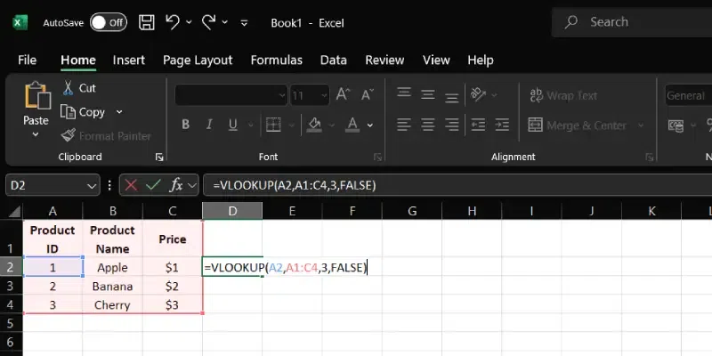
- **Select a Cell for the Result: Click in the cell where we want the VLOOKUP result to appear, here we select D2.
- **Start the Formula: Type
=VLOOKUP(in cell D2, and begin building the formula using the lookup value from another cell (for example, A2).
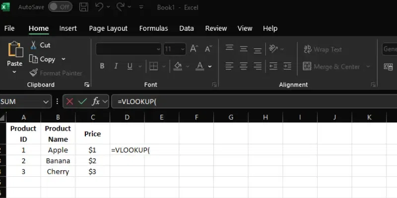
Enter the VLOOKUP Formula
Step 3: Define the Lookup Value
Enter the value we want to search for in the formula:
- Use a cell reference, like
A2, or type a value directly in quotes, such as"001". - Example: If searching for a product ID in cell D2, start the formula as:
=VLOOKUP(A2, or =VLOOKUP("001", - Add a comma after the lookup value to move to the next part of the formula.
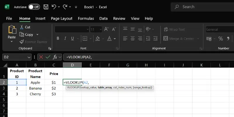
Define the Lookup Value
Step 4: Specify the Table Array
We define the range where VLOOKUP searches for our data, ensuring it includes all relevant columns. This step is crucial for accurate results, as it tells Excel exactly where to look. Let’s set it up carefully to match our table structure.
- Select the data range where we want to search, e.g., A1:C4(IDs in column A and Prices in column C).
- Highlight the range by clicking and dragging.
- Add a comma after selecting the table array.
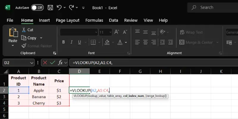
Specify the Table Array
Step 5: Indicate the Column Index Number
We choose the column from which VLOOKUP retrieves our data, a critical decision for accurate results. This number tells Excel where to pull the information once a match is found. Let’s select it with precision to match our table layout.
- Enter the column number from which we want to retrieve the data.
- For example, if prices are in the third column (C), type 3 in the formula: =VLOOKUP(D2, A1:C4, 3,.
- Add a comma after the column number.
**Purpose of col_index_num:
The col_index_num in a VLOOKUP formula specifies which column in the table_array to pull the data from, once a match is found for the lookup_value in the first column of that array.
**Importance of the Column Index Number:
In the range A1:C4:
- **Column A: Product IDs
- **Column B: Product Names
- **Column C: Prices
The column index number (3) tells Excel to return data from the third column (Prices) of the table when a match is found in the first column. This ensures VLOOKUP retrieves the correct information.
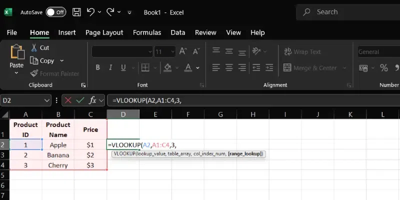
Indicate the Column Index Number
Step 6: Choose the Range Lookup Type
The range_lookup decides how VLOOKUP matches data:
- **FALSE: Exact match. Returns a value only if the lookup value exists; otherwise shows #N/A. Recommended for precise searches like Product IDs or prices.
- **TRUE: Approximate match, used for sorted data.
Using FALSE ensures accuracy, retrieving the exact corresponding value and avoiding errors from approximate matches.
Choose the Range Lookup Type
Step 7: Complete and Execute the Formula
We finalize our VLOOKUP formula and see the results come to life in our spreadsheet. This step confirms our setup works, delivering the data we need. Let’s execute it with confidence.
**1. Press Enter: Our complete formula in cell D2 should look like this:
=VLOOKUP(A2, A1:C4, 3, FALSE)
**2.**View the Result: After pressing Enter, cell D2 should display $1, which is the price of the product with ID 001.
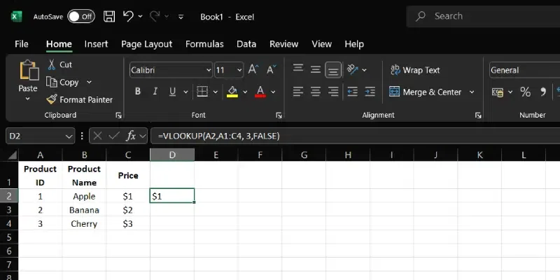
Complete and Execute the Formula
VLOOKUP Between Two Excel Spreadsheets
Using the VLOOKUP function to connect data between two Excel sheets within the same workbook is an efficient way to improve efficiency and smooth our workflow. Here’s an easy step-by-step guide to help us use VLOOKUP across two sheets.
Example****:**
Imagine we have an Excel workbook with two sheets.
Sheet1 ("Employee Info") contains a list of employee IDs and their names.
| Employee ID | Employee Name |
|---|---|
| 101 | John Doe |
| 102 | Jane Smith |
| 103 | Emily White |
Sheet2 ("Contact Details") contains a list of employee IDs and their corresponding email addresses.
| Employee ID | |
|---|---|
| 101 | john.doe@email.com |
| 102 | jane.smith@email.com |
| 103 | emily.white@email.com |
Goal
Use VLOOKUP to display employee email addresses in Sheet1 based on their IDs.
Step 1: Set Up VLOOKUP in Sheet1
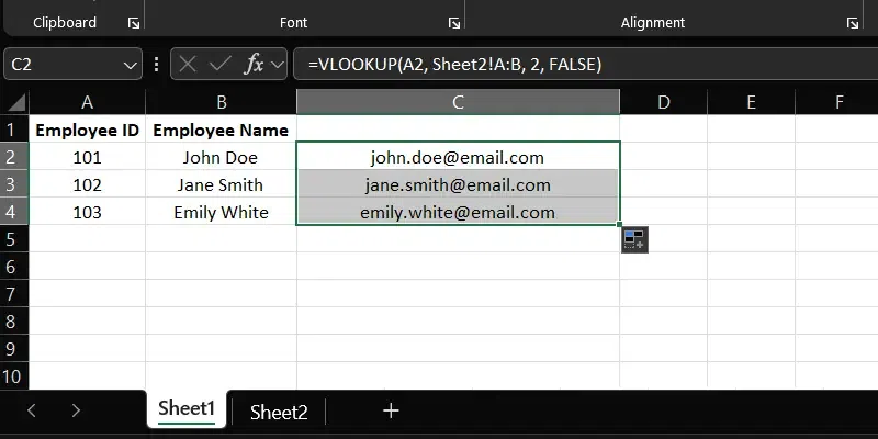
Navigate to Sheet1 ("Employee Info") and click on cell C2 (right next to the first Employee ID).
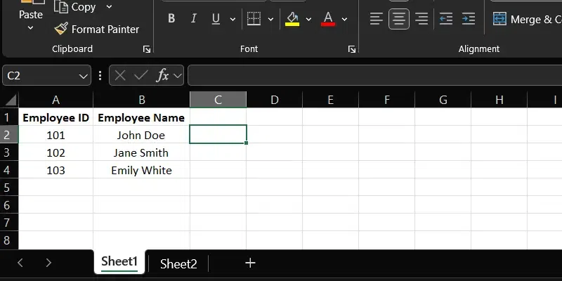
Set Up VLOOKUP in Sheet1
Step 2: Enter the VLOOKUP Formula
Type in the following formula in cell C2 of Sheet1:
**Syntax:
=VLOOKUP(A2, Sheet2!A:B, 2, FALSE)
Here’s a simple explanation of each part of the formula:
- **A2: Refers to the cell in Sheet1 containing the Employee ID we want to look up.
- **Sheet2!A:B: Tells Excel to search in columns A to B of Sheet2. The "Sheet2!" notation indicates the data is on another sheet.
- **2: Specifies that the result we want (the email address) is in the second column of the range in Sheet2.
- **FALSE: Ensures the formula returns an exact match for the Employee ID.
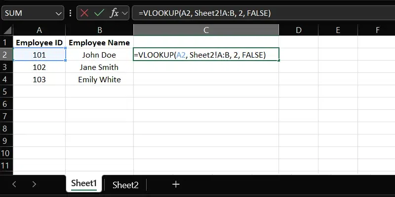
Enter the VLOOKUP Formula
Step 3: Apply and Copy the Formula
We bring our VLOOKUP formula to life and extend it across our data, ensuring all rows update correctly. This step links our sheets seamlessly, saving us time. Let’s apply it with care.
- **Press Enter: After typing the formula in cell C2, press Enter. The result, "john.doe@email.com" will appear for Employee ID 101.
- **Copy the Formula: Click on cell C2.
- **Drag the Fill Handle: Use the small square at the bottom-right corner of the cell. Drag it down to copy the formula to the other cells in Column C.
- **Auto-Adjust: Excel will automatically adjust the formula for each row, showing the corresponding email addresses for the other Employee IDs (C3, C4, etc).
Execute and Extend the Formula
Step 4: Verify the Results
- Check that the correct email addresses appear next to the corresponding employee names in Sheet1.
VLOOKUP Between Two Workbooks
VLOOKUP is a prominent tool that can pull data from one workbook to another, making it easy to consolidate and analyze information stored in separate files. Here’s a step-by-step guide on how to use VLOOKUP across two Excel workbooks.
Example
- Suppose we're working with sales data and we have two Excel workbooks:
- Workbook2 (“Employee Sales.xlsx”) contains data in Sheet1 with Transaction IDs and employee names.
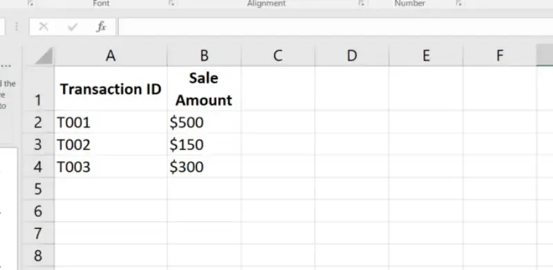
Prepare your Data in Sheet1
- Workbook2 ("Employee Sales.xlsx") contains Transaction IDs and the corresponding employee names who made the sales.
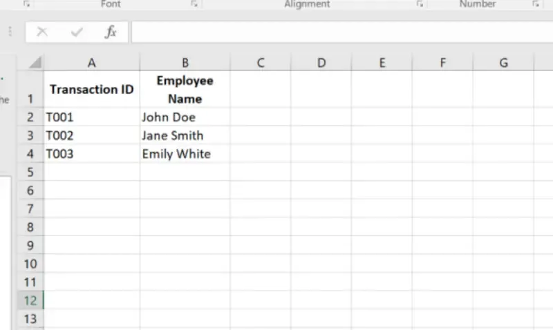
Prepare your Data in Sheet2
Goal
- We want to add a third column to the "Sales Data.xlsx" workbook that displays each employee's name associated with the transactions by linking the data using the Transaction ID.
Step 1: Open Both Workbooks
We begin by accessing the files we need to link, setting the foundation for our VLOOKUP. This ensures all data is ready for seamless integration across workbooks. Let’s open them with purpose.
- Open "Sales Data.xlsx" (Workbook1) and "Employee Sales.xlsx" (Workbook2) simultaneously.
- This ensures Excel can reference the second workbook while creating the VLOOKUP formula.
Step 2: Set Up VLOOKUP in Workbook1
We prepare our primary workbook to apply VLOOKUP, starting with the right cell. This step positions us to link data accurately from the second file. Let’s set it up carefully.
- Go to Workbook1 ("Sales Data.xlsx").
- Select cell C2 (next to the first Transaction ID).
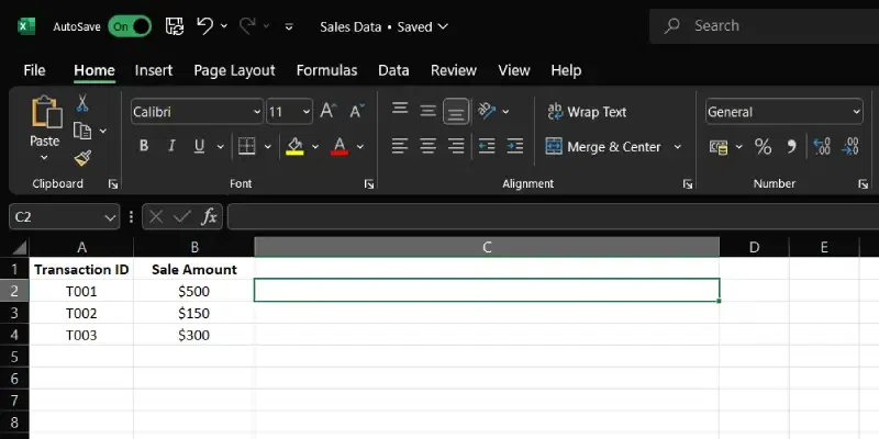
Set Up VLOOKUP in Workbook1
Step 3: Enter the VLOOKUP Formula
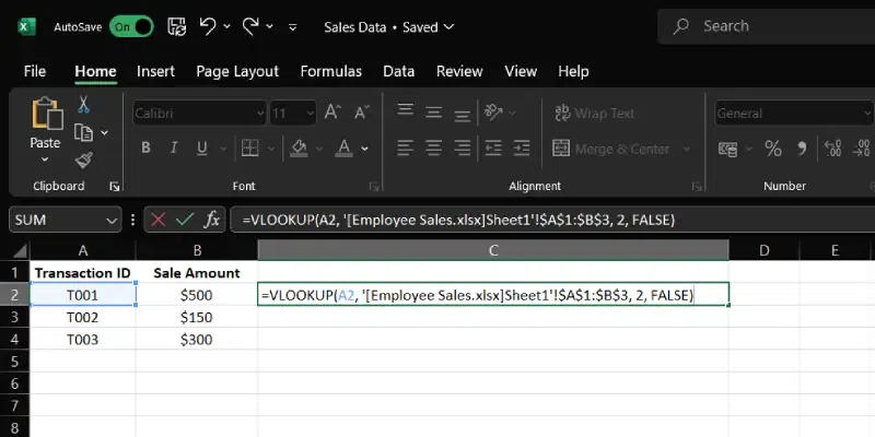
Type in the following formula in cell C2 of "Sales Data.xlsx":
=VLOOKUP(A2, '[Employee Sales.xlsx]Sheet1'!$A$1:$B$3, 2, FALSE)
**Understanding the VLOOKUP Formula:
- **A2: Lookup value (Transaction ID in "Sales Data.xlsx").
- ****'[Employee Sales.xlsx]Sheet1'!$A$1:$B$3**: Table array in the other workbook; $ keeps the range fixed when copied.
- **2: Column number to return (Employee Name).
- **FALSE: Exact match for the Transaction ID.
Enter the VLOOKUP Formula in Sales Data Workbook
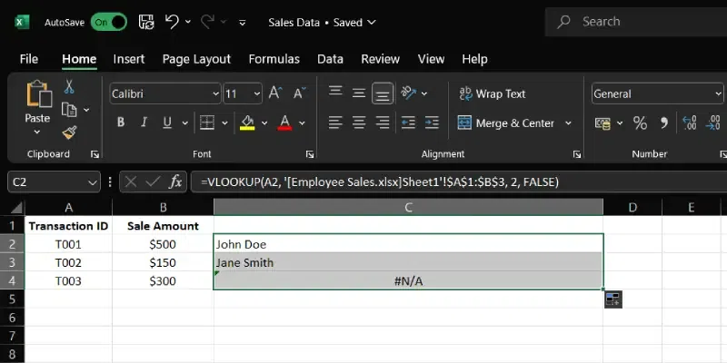
Step 4: Execute and Extend the Formula
Press Enter to execute the formula in cell C2. If correctly entered, cell C2 will now display "John Doe", corresponding to Transaction ID T001.
To apply the same formula to the other transactions:
- Click on cell C2.
- Drag the fill handle down through the column to fill the rest of the cells in Column C with the VLOOKUP formula, adjusting it for the subsequent rows (C3, C4, etc.).
Execute and Extend the Formula
Step 5: Verify the Results
Check that the correct employee names appear next to the corresponding transaction IDs in "Sales Data.xlsx".