Backpropagation in Neural Network (original) (raw)
Last Updated : 12 May, 2026
Backpropagation is an algorithm that trains neural networks by reducing prediction error. It works by propagating errors backward, computing gradients using the chain rule, and updating weights and biases to improve performance.
- Computes gradients of the loss function with respect to each weight using the chain rule
- Updates weights and biases efficiently to reduce error
- Scales well to deep and complex neural networks
- Enables automatic learning and continuous improvement across training iterations

Fig(a) A simple illustration of how the backpropagation works by adjustments of weights
Working of Back Propagation Algorithm
The Back Propagation algorithm involves two main steps:
1. Forward Pass Work
In forward pass, input data moves through the network to generate an output.
- Input data is passed to the input layer and forwarded to hidden layers
- Each neuron computes a weighted sum and adds a bias
- Activation functions (like ReLU) are applied to produce outputs
- Outputs from one layer become inputs to the next layer
- Final layer uses functions like softmax to produce predictions (e.g., probabilities for classification)

The forward pass using weights and biases
2. Backward Pass
In this step, the error between predicted and actual output is propagated backward to update weights and biases. Error is calculated (e.g., using Mean Squared Error)
\text{MSE} = (\text{Predicted Output} - \text{Actual Output})^2
- Gradients are computed using the chain rule
- Weights and biases are updated to reduce the error
- Process continues layer by layer from output to input
- Derivatives of activation functions are used to compute gradients effectively
Example
Let’s walk through an example of Back Propagation in machine learning. Assume the neurons use the sigmoid activation function for the forward and backward pass. The target output is 0.5 and the learning rate is 1.

Example (1) of backpropagation sum
Forward Propagation
1. Initial Calculation
The weighted sum at each node is calculated using:
a j =∑(w i ,j∗x i )
Where,
- a_j is the weighted sum of all the inputs and weights at each node
- w_{i,j} represents the weights between the i^{th}input and the j^{th} neuron
- x_i represents the value of the i^{th} input
**O (output): After applying the activation function to a, we get the output of the neuron:
o_j = activation function(a_j )
2. Sigmoid Function
The sigmoid function returns a value between 0 and 1, introducing non-linearity into the model.
y_j = \frac{1}{1+e^{-a_j}}

To find the outputs of y3, y4 and y5
3. Computing Outputs
At h1 node
\begin {aligned}a_1 &= (w_{1,1} x_1) + (w_{2,1} x_2) \\& = (0.2 * 0.35) + (0.2* 0.7)\\&= 0.21\end {aligned}
Once we calculated the a1 value, we can now proceed to find the y3 value:
y_j= F(a_j) = \frac 1 {1+e^{-a_1}}
y_3 = F(0.21) = \frac 1 {1+e^{-0.21}}
y_3 = 0.56
Similarly find the values of y4 at **h 2 and y5 at O3
a_2 = (w_{1,2} * x_1) + (w_{2,2} * x_2) = (0.3*0.35)+(0.3*0.7)=0.315
y_4 = F(0.315) = \frac 1{1+e^{-0.315}}
a3 = (w_{1,3}*y_3)+(w_{2,3}*y_4) =(0.3*0.57)+(0.9*0.59) =0.702
y_5 = F(0.702) = \frac 1 {1+e^{-0.702} } = 0.67

Values of y3, y4 and y5
4. Error Calculation
Our actual output is 0.5 but we obtained 0.67__._ To calculate the error we can use the below formula:
Error_j= y_{target} - y_5
\text{=>} \space 0.5 - 0.67 = -0.17
Using this error value we will be backpropagating.
**Back Propagation
**1. Calculating Gradients
The change in each weight is calculated as:
\Delta w_{ij} = \eta \times \delta_j \times O_j
Where:
- \delta_j is the error term for each unit,
- \eta is the learning rate.
**2. Output Unit Error
For O3:
\delta_5 = y_5(1-y_5) (y_{target} - y_5)
= 0.67(1-0.67)(-0.17) = -0.0376
**3. Hidden Unit Error
For h1:
\delta_3 = y_3 (1-y_3)(w_{1,3} \times \delta_5)
= 0.56(1-0.56)(0.3 \times -0.0376) = -0.0027
For h2:
\delta_4 = y_4(1-y_4)(w_{2,3} \times \delta_5)
=0.59 (1-0.59)(0.9 \times -0.0376) = -0.00819
4. Weight Updates
For the weights from hidden to output layer:
\Delta w_{2,3} = 1 \times (-0.0376) \times 0.59 = -0.022184
New weight:
w_{2,3}(\text{new}) = -0.022184 + 0.9 = 0.877816
For weights from input to hidden layer:
\Delta w_{1,1} = 1 \times (-0.0027) \times 0.35 = -0.000945
New weight:
w_{1,1}(\text{new}) = - 0.000945 + 0.2 = 0.199055
Similarly other weights are updated:
- w_{1,2}(\text{new}) = 0.273225
- w_{1,3}(\text{new}) = 0.086615
- w_{2,1}(\text{new}) = 0.269445
- w_{2,2}(\text{new}) = 0.18534
The updated weights are illustrated below
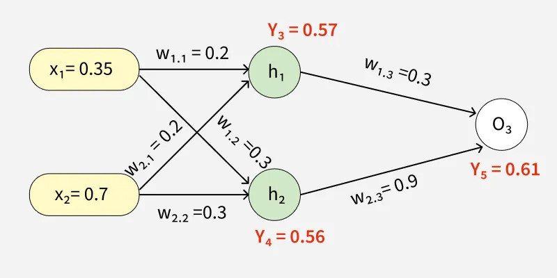
Through backward pass the weights are updated
After updating the weights the forward pass is repeated hence giving:
- y_3 = 0.57
- y_4 = 0.56
- y_5 = 0.61
Since y_5 = 0.61 is still not the target output the process of calculating the error and backpropagating continues until the desired output is reached.
This process demonstrates how Back Propagation iteratively updates weights by minimizing errors until the network accurately predicts the output.
Error = y_{target} - y_5
= 0.5 - 0.61 = -0.11
This process is said to be continued until the actual output is gained by the neural network.
Back Propagation Implementation in Python for XOR Problem
This code demonstrates how Back Propagation is used in a neural network to solve the XOR problem. The neural network consists of:
1. Defining Neural Network
The network consists of 2 input neurons, 4 hidden neurons and 1 output neuron, using the sigmoid activation function.
- input_size and hidden_size define the layer sizes
- weights_input_hidden initializes weights from input to hidden layer
- weights_hidden_output initializes weights from hidden to output layer
- bias_hidden and bias_output initialize bias terms for respective layers Python `
import numpy as np
class NeuralNetwork: def init(self, input_size, hidden_size, output_size): self.input_size = input_size self.hidden_size = hidden_size self.output_size = output_size
    self.weights_input_hidden = np.random.randn(
        self.input_size, self.hidden_size)
    self.weights_hidden_output = np.random.randn(
        self.hidden_size, self.output_size)

    self.bias_hidden = np.zeros((1, self.hidden_size))
    self.bias_output = np.zeros((1, self.output_size))

def sigmoid(self, x):
    return 1 / (1 + np.exp(-x))

def sigmoid_derivative(self, x):
    return x * (1 - x)
`
2. Defining Feed Forward Network
In Forward pass inputs are passed through the network activating the hidden and output layers using the sigmoid function.
- Computes hidden layer activation using weighted sum and bias
- Applies sigmoid to get hidden layer output
- Computes output layer activation from hidden outputs
- Applies sigmoid to produce final predicted output Python `
def feedforward(self, X): self.hidden_activation = np.dot( X, self.weights_input_hidden) + self.bias_hidden self.hidden_output = self.sigmoid(self.hidden_activation)
self.output_activation = np.dot(
    self.hidden_output, self.weights_hidden_output) + self.bias_output
self.predicted_output = self.sigmoid(self.output_activation)

return self.predicted_output
`
3. Defining Backward Network
In the backward pass, the network calculates the error and updates weights using gradients from the sigmoid function.
- Computes output error as difference between actual and predicted values
- Calculates output delta using sigmoid derivative
- Propagates error to hidden layer using dot product
- Computes hidden delta using sigmoid derivative
- Updates weights between hidden output and input hidden layers Python `
def backward(self, X, y, learning_rate):
output_error = y - self.predicted_output
output_delta = output_error *
self.sigmoid_derivative(self.predicted_output)
hidden_error = np.dot(output_delta, self.weights_hidden_output.T)
hidden_delta = hidden_error * self.sigmoid_derivative(self.hidden_output)

self.weights_hidden_output += np.dot(self.hidden_output.T,
                                     output_delta) * learning_rate
self.bias_output += np.sum(output_delta, axis=0,
                           keepdims=True) * learning_rate
self.weights_input_hidden += np.dot(X.T, hidden_delta) * learning_rate
self.bias_hidden += np.sum(hidden_delta, axis=0,
                           keepdims=True) * learning_rate
`
4. Training Network
The network is trained over 10,000 epochs using the Back Propagation algorithm with a learning rate of 0.1 progressively reducing the error.
- **output = self.feedforward(X): computes the output for the current inputs
- **self.backward(X, y, learning_rate): updates weights and biases using Back Propagation
- **loss = np.mean(np.square(y - output)): calculates the mean squared error (MSE) loss Python `
def train(self, X, y, epochs, learning_rate): for epoch in range(epochs): output = self.feedforward(X) self.backward(X, y, learning_rate) if epoch % 4000 == 0: loss = np.mean(np.square(y - output)) print(f"Epoch {epoch}, Loss:{loss}")
`
5. Testing Neural Network
- **X = np.array([[0, 0], [0, 1], [1, 0], [1, 1]]): defines the input data
- **y = np.array([[0], [1], [1], [0]]): defines the target values
- **nn = NeuralNetwork(input_size=2, hidden_size=4, output_size=1): initializes the neural network
- **nn.train(X, y, epochs=10000, learning_rate=0.1): trains the network
- **output = nn.feedforward(X): gets the final predictions after training Python `
X = np.array([[0, 0], [0, 1], [1, 0], [1, 1]]) y = np.array([[0], [1], [1], [0]])
nn = NeuralNetwork(input_size=2, hidden_size=4, output_size=1) nn.train(X, y, epochs=10000, learning_rate=0.1)
output = nn.feedforward(X) print("Predictions after training:") print(output)
`
**Output:

Trained Model
Download full code from here
Advantages
- Easy to implement and beginner-friendly, as it updates weights using error derivatives
- Simple and flexible, making it suitable for different types of networks like feedforward, CNNs, and RNNs
- Efficient in learning, as it directly adjusts weights based on error, especially in deep networks
- Helps models generalize well, improving performance on unseen data
- Scales effectively with large datasets and complex architectures
Challenges
- Gradients can become very small in deep networks, making learning slow or difficult (vanishing gradient problem)
- Gradients can grow too large, causing unstable training and divergence (exploding gradients)
- Complex models may overfit the training data instead of learning general patterns