Box Office Revenue Prediction Using Linear Regression in ML (original) (raw)
Last Updated : 23 Jul, 2025
The objective of this project is to develop a machine learning model using Linear Regression to accurately predict the box office revenue of movies based on various available features. The model will be trained on a dataset containing historical movie data and will aim to identify key factors that impact revenue. By implementing data preprocessing, feature engineering, visualization and model evaluation techniques, this project seeks to:
- Build a predictive model that can estimate the expected revenue of a movie prior to its release.
- Provide insights into which features most influence box office success.
- Compare linear regression performance with more advanced models (e.g., XGBoost) to assess predictive accuracy.
1. Importing Libraries and Dataset
Core Libraries
- **Pandas: For loading and exploring the dataset.
- **NumPy:For working with numerical arrays and math operations.
Visualization
- **Matplotlib and **Seaborn****:** Used to plot data distributions, trends and model performance.
Preprocessing and Modeling
- **train_test_split: Splits the data into training and validation sets.
- **LabelEncoder: Converts categories like genres into numeric format.
- **StandardScaler: Scales features for better model performance.
- **CountVectorizer: Converts text data (e.g., genres) into numeric vectors.
- **metrics: Offers tools for evaluating model accuracy.
Advanced Modeling
- **XGBoost****:** A high-performance gradient boosting algorithm used for better predictions.
Utility
- **warnings.filterwarnings('ignore'): Hides unnecessary warning messages for cleaner output. Python `
import numpy as np import pandas as pd import matplotlib.pyplot as plt import seaborn as sb from sklearn.model_selection import train_test_split from sklearn.preprocessing import LabelEncoder, StandardScaler from sklearn.feature_extraction.text import CountVectorizer from sklearn import metrics from xgboost import XGBRegressor
import warnings warnings.filterwarnings('ignore')
`
2. Loading the dataset into a pandas DataFrame
We now load the dataset into a pandas DataFrame to begin analysis. You can download the dataset from **here.
Python `
df = pd.read_csv('boxoffice.csv', encoding='latin-1') df.head()
`
**Output:
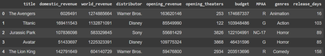
df.head()
2.1 Checking Dataset Size
Let's see how many rows and columns we have.
Python `
df.shape
`
**Output:
(2694, 10)
2.2 Checking Data Types
We check the data types of each column and look for issues.
Python `
df.info()
`
**Output:
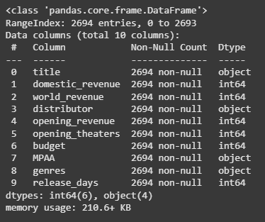
Checking Data Types
Here we can observe an unusual discrepancy in the dtype column the columns which should be in the number format are also in the object type. This means we need to clean the data before moving any further.
3. Exploring the Dataset
We take a quick look at statistical metrics (like mean, min, max) for each numeric column to understand the data distribution.
- **df.describe() gives a summary of the numeric columns (count, mean, standard deviation, min, max, etc.).
- ****.T** transposes the output for better readability ( rows become columns and vice versa ). Python `
df.describe().T
`
**Output:
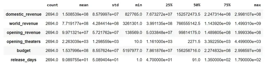
Statistical Summary
Since we are predicting only domestic revenue in this project, we are dropping **world_revenue and **opening_revenue columns from the dataframe.
Python `
to_remove = ['world_revenue', 'opening_revenue'] df.drop(to_remove, axis=1, inplace=True)
`
3.1 Checking Missing Values
We calculate what percentage of values is missing in each column. **isnull().sum() functions helps us identify columns with many missing entries.
Python `
df.isnull().sum() * 100 / df.shape[0]
`
**Output:
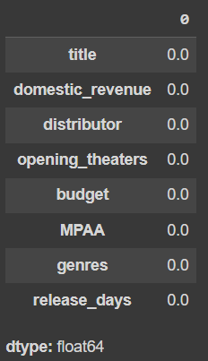
percentage of entries in each column that is null
4. Handling Missing Values
We clean the data by removing or filling missing values appropriately.
- We drop the budget column entirely, likely due to too many missing values.
- Fill missing values in MPAA and genres columns using their most frequent values (mode).
- Remove any remaining rows with missing values.
- Finally, check if any null values remain; the result should be 0. Python `
df.drop('budget', axis=1, inplace=True)
for col in ['MPAA', 'genres']: df[col] = df[col].fillna(df[col].mode()[0])
df.dropna(inplace=True)
df.isnull().sum().sum()
`
**Output:
0
**4.1 Cleaning Numeric Columns Stored as Strings
Some numeric columns might be stored as strings with special characters (like $ or ,). We need to remove these characters and convert the columns back to numeric format.
- Remove the first character from '**domestic_revenue' (likely a $ sign).
- Remove commas from numeric values (e.g., 1,000 to 1000).
- Ensure the columns are properly converted to float types.
- Use **pd.to_numeric to handle any remaining non-numeric values gracefully to turn them into **NaNs. Python `
df['domestic_revenue'] = df['domestic_revenue'].astype(str).str[1:]
for col in ['domestic_revenue', 'opening_theaters', 'release_days']: df[col] = df[col].astype(str).str.replace(',', '')
temp = (~df[col].isnull())
df[temp][col] = df[temp][col].convert_dtypes(float)

df[col] = pd.to_numeric(df[col], errors='coerce')
`
5. **Visualizing MPAA Rating Distribution
We want to see how many movies fall under each MPAA rating category like PG, R, PG-13, etc. We will create a horizontal bar chart showing the count of movies in each MPAA rating.
- **plt.figure(figsize=(10, 5)) sets the size of the plot.
- **sb.countplot() from Seaborn automatically counts and plots the frequency of each category in the 'MPAA' column.
- **plt.show() displays the plot. Python `
plt.figure(figsize=(10, 5)) sb.countplot(df['MPAA']) plt.show()
`
**Output:
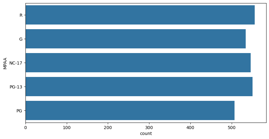
countplot
**5.1 Average Domestic Revenue by MPAA Rating
We group the dataset by the 'MPAA' rating category and calculate the mean (average) of the '**domestic_revenue' for each rating group.
Python `
df.groupby('MPAA')['domestic_revenue'].mean()
`
**Output:
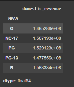
Average Domestic Revenue by MPAA Rating
Here we can observe that the movies with PG or R ratings generally have their revenue higher than the other rating class.
**6. Visualizing Distributions of Key Numeric Features
We plot the distribution (shape) of three important numeric columns to see how their values spread out.
- We create three side-by-side plots in one row.
- For each feature (domestic_revenue, opening_theaters, release_days) we show the distribution using Seaborn’s distplot.
- This helps check if the data is normally distributed, skewed or has any unusual patterns. Python `
plt.subplots(figsize=(15, 5))
features = ['domestic_revenue', 'opening_theaters', 'release_days'] for i, col in enumerate(features): plt.subplot(1, 3, i+1) sb.distplot(df[col]) plt.tight_layout() plt.show()
`
**Output:
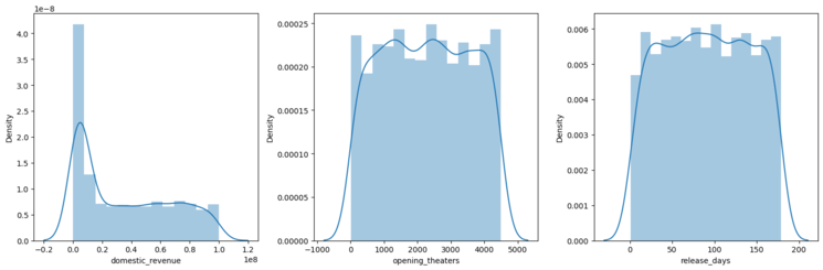
distplot
Understanding these distributions is important before modeling, as it affects how the model interprets the data.
**7. Detecting Outliers Using Boxplots
We use boxplots to visually check for outliers in key numeric features. Boxplots show the spread of data and highlight any outliers (points outside the whiskers).
- We create three boxplots side by side, one for each feature (domestic_revenue, opening_theaters, release_days).
- This helps us identify unusual values that might affect the model. Python `
plt.subplots(figsize=(15, 5)) for i, col in enumerate(features): plt.subplot(1, 3, i+1) sb.boxplot(df[col]) plt.tight_layout() plt.show()
`
**Output:
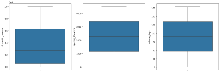
Outliers
We can observe that there are no outliers in the above features.
**8. Applying Log Transformation to Numeric Features
We apply a log transformation to reduce skewness in our numeric data because log transformation often improves model performance and stability.
- We take the base-10 logarithm of each value in the specified columns (domestic_revenue, opening_theaters, release_days).
- This helps make skewed data more normally distributed and reduces the effect of extreme values. Python `
for col in features: df[col] = df[col].apply(lambda x: np.log10(x))
`
Now the data in the columns we have visualized above should be close to normal distribution.
**8.1 Checking Distributions After Log Transformation
We visualize the distributions of the numeric features again to see the effect of the log transformation.
Python `
plt.subplots(figsize=(15, 5)) for i, col in enumerate(features): plt.subplot(1, 3, i+1) sb.distplot(df[col]) plt.tight_layout() plt.show()
`
**Output:
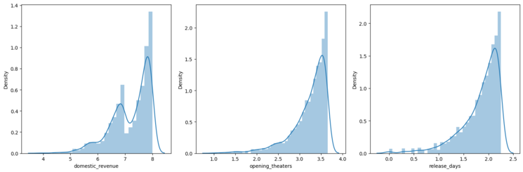
Normal Distribution
**9. Converting Movie Genres into Numeric Features
We transform the text data in the genres column into separate numeric features using one-hot encoding.
- We use **CountVectorizer to convert each genre like “Action”, “Comedy” into a binary feature i.e 1 if the movie belongs to that genre, else 0.
- Then drop the original genres text column since it’s now represented numerically. Python `
vectorizer = CountVectorizer() vectorizer.fit(df['genres']) features = vectorizer.transform(df['genres']).toarray()
genres = vectorizer.get_feature_names_out() for i, name in enumerate(genres): df[name] = features[:, i]
df.drop('genres', axis=1, inplace=True)
`
But there will be certain genres that are not that frequent which will lead to increases in the complexity of the model unnecessarily. So we will remove those genres which are very rare.
**9.1 Removing Rare Genre Columns with Mostly Zero Values
We will check for columns between 'action' and 'western' in the DataFrame and drop columns where over 95% of values are zero meaning that genre is rare.
Python `
removed = 0
if 'action' in df.columns and 'western' in df.columns: for col in df.loc[:, 'action':'western'].columns:
    if (df[col] == 0).mean() > 0.95:
        removed += 1
        df.drop(col, axis=1, inplace=True)
print(removed) print(df.shape)
`
**Output:
0
(2694, 12)
This helps simplify the model by focusing on genres that actually appear frequently.
10. Encoding Categorical Columns into Numbers
We use **LabelEncoderto replace each unique category with a number like “PG” to 0, “R” to 1. This is necessary because machine learning models work better with numbers than text labels.
Python `
for col in ['distributor', 'MPAA']: le = LabelEncoder() df[col] = le.fit_transform(df[col])
`
**11. Visualizing Strong Correlations Between Numeric Features
As all the categorical features have been labeled encoded let's check if there are highly correlated features in the dataset.
- We will calculate the correlation matrix for all numeric columns.
- The plot a heatmap, highlighting pairs of features with correlation greater than 0.8 (very strong correlation).
This helps us identify redundant features that may need to be removed or handled before modeling.
Python `
plt.figure(figsize=(8, 8)) sb.heatmap(df.select_dtypes(include=np.number).corr() > 0.8, annot=True, cbar=False) plt.show()
`
**Output:
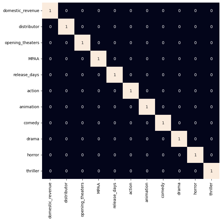
heatmap
**12. Preparing Data for Model Training and Validation
Now we will separate the features and target variables and split them into training and the testing data by using which we will select the model which is performing best on the validation data.
- We will remove the title and target column **domestic_revenue from the features and set **domestic_revenue as the target variable.
- We split the data into 90% training and 10% validation sets to evaluate model performance. Python `
features = df.drop(['title', 'domestic_revenue'], axis=1) target = df['domestic_revenue'].values
X_train, X_val, Y_train, Y_val = train_test_split(features, target, test_size=0.1, random_state=22) X_train.shape, X_val.shape
`
**Output:
((2424, 10), (270, 10))
**12.1 Normalizing Features for Better Model Training
We scale the features to have a mean of 0 and a standard deviation of 1, which helps models learn more effectively.
- **fit_transform learns scaling parameters from training data and applies scaling.
- transform applies the same scaling to validation data without changing the scaler.
This standardization helps the model converge faster and improves stability during training.
Python `
scaler = StandardScaler() X_train = scaler.fit_transform(X_train) X_val = scaler.transform(X_val)
`
**13. Training the XGBoost Regression Model
XGBoost library models help to achieve state-of-the-art results most of the time so, we will also train this model to get better results.
- We initialize an **XGBoost regressor a gradient boosting model.
- Then train the model on the normalized training data (**X_train) and target values (**Y_train). Python `
from sklearn.metrics import mean_absolute_error as mae model = XGBRegressor() model.fit(X_train, Y_train)
`
**14. Evaluating Model Performance on Training and Validation Sets
We use Mean Absolute Error (MAE) to check how well the model predicts revenue on both training and validation data.
- We predict revenue for the training data and calculate MAE to measure training error.
- Also we predict revenue for the validation data and calculate MAE to measure how well the model generalizes.
**Note: Lower MAE means better predictions, it helps identify if the model is overfitting or underfitting.
Python `
train_preds = model.predict(X_train) print('Training Error : ', mae(Y_train, train_preds))
val_preds = model.predict(X_val) print('Validation Error : ', mae(Y_val, val_preds)) print()
`
**Output:
Training Error: 0.2104541861999253
Validation Error: 0.6358190127903746
We can observe that :
- **Training Error (0.21) is low: The model fits the training data quite well.
- **Validation Error (0.63) is significantly higher than training: This gap suggests the model might be overfitting, meaning it performs well on training data but not as well on unseen (validation) data.
Get the Complete notebook:
**Notebook: **click here.