XGBoost (original) (raw)

Last Updated : 19 Mar, 2026

Traditional models like decision trees and random forests are easy to interpret but may lack accuracy on complex data. XGBoost (eXtreme Gradient Boosting) is an optimized gradient boosting algorithm that combines multiple weak models into a stronger, high-performance model.

• It uses decision trees as base learners, building them sequentially so each tree corrects errors from the previous one and it is known as boosting.
• It features parallel processing for faster training on large datasets and allows parameter customization to optimize performance for specific problems.

How XGBoost Works?

It builds decision trees sequentially with each tree attempting to correct the mistakes made by the previous one. The process can be broken down as follows:

1. **Start with a base learner: The first model decision tree is trained on the data. In regression tasks this base model simply predicts the average of the target variable.
2. **Calculate the errors: After training the first tree the errors between the predicted and actual values are calculated.
3. **Train the next tree: The next tree is trained on the errors of the previous tree. This step attempts to correct the errors made by the first tree.
4. **Repeat the process: This process continues with each new tree trying to correct the errors of the previous trees until a stopping criterion is met.
5. **Combine the predictions: The final prediction is the sum of the predictions from all the trees.

Mathematics Behind XGBoost Algorithm

It can be viewed as iterative process where we start with an initial prediction often set to zero. After which each tree is added to reduce errors. Mathematically the model can be represented as:

\hat{y}_{i} = \sum_{k=1}^{K} f_k(x_i)

Where:

• \hat{y}_{i} is the final predicted value for the i^{th} data point
• K is the number of trees in the ensemble
• f_k(x_i) represents the prediction of the K^{th} tree for the i^{th} data point.

The objective function in XGBoost consists of two parts i.e a loss function and a regularization term. The loss function measures how well the model fits the data and the regularization term simplify complex trees. The general form of the loss function is:

obj(\theta) = \sum_{i}^{n} l(y_{i}, \hat{y}_{i}) + \sum_{k=1}^K \Omega(f_{k}) \\

Where:

• l(y_{i}, \hat{y}_{i}) is the loss function which computes the difference between the true value y_i​ and the predicted value \hat{y}_i,
• \Omega(f_{k}) \\ is the regularization term which discourages overly complex trees.

Now instead of fitting the model all at once we optimize the model iteratively. We start with an initial prediction \hat{y}_i^{(0)} =0 and at each step we add a new tree to improve the model. The updated predictions after adding the t^{th} tree can be written as:

\\ \hat{y}_i^{(t)} = \hat{y}_i^{(t-1)} + f_t(x_i)

Where:

• \hat{y}_i^{(t-1)} is the prediction from the previous iteration
• f_t(x_i) is the prediction of the t^{th} tree for the i^{th} data point.

The regularization term \Omega(f_t) simplify complex trees by penalizing the number of leaves in the tree and the size of the leaf. It is defined as:

\Omega(f_t) = \gamma T + \frac{1}{2}\lambda \sum_{j=1}^T w_j^2

Where:

• \Tau is the number of leaves in the tree
• \gamma is a regularization parameter that controls the complexity of the tree
• \lambda is a parameter that penalizes the squared weight of the leaves w_j​

Finally, when deciding how to split the nodes in the tree we compute the information gain for every possible split. The information gain for a split is calculated as:

Gain = \frac{1}{2} \left[\frac{G_L^2}{H_L+\lambda}+\frac{G_R^2}{H_R+\lambda}-\frac{(G_L+G_R)^2}{H_L+H_R+\lambda}\right] - \gamma

Where:

• G_L, G_R are the sums of gradients in the left and right child nodes
• H_L, H_R are the sums of Hessians in the left and right child nodes

By calculating the information gain for every possible split at each node XGBoost selects the split that results in the largest gain which effectively reduces the errors and improves the model's performance.

How XGBoost Improves Traditional Gradient Boosting

XGBoost extends traditional gradient boosting by including regularization elements in the objective function, XGBoost improves generalization and prevents overfitting.

1. Preventing Overfitting

XGBoost incorporates several techniques to reduce overfitting and improve model generalization:

• **Learning rate (eta): Controls each tree’s contribution i.e a lower value makes the model more conservative.
• **Regularization: Adds penalties to complexity to prevent overly complex trees.
• **Pruning: Trees grow depth-wise and splits that do not improve the objective function are removed, keeping trees simpler and faster.
• **Combination effect: Using learning rate, regularization and pruning together enhances robustness and reduces overfitting.

2. Tree Structure

XGBoost builds trees level-wise (breadth-first) rather than the conventional depth-first approach, adding nodes at each depth before moving to the next level.

• **Best splits: Evaluates every possible split for each feature at each level and selects the one that minimizes the objective function like MSE for regression and cross-entropy for classification.
• **Feature prioritization: Level-wise growth reduces overhead, as all features are considered simultaneously, avoiding repeated evaluations.
• **Benefit: Handles complex feature interactions effectively by considering all features at the same depth.

3. Handling Missing Data

XGBoost manages missing values robustly during training and prediction using a sparsity-aware approach.

• **Sparsity-Aware Split Finding: Treats missing values as a separate category when evaluating splits.
• **Default direction: During tree building, missing values follow a default branch.
• **Prediction: Instances with missing features follow the learned default branch.
• **Benefit: Ensures robust predictions even with incomplete input data.

4. Cache-Aware Access

XGBoost optimizes memory usage to speed up computations by taking advantage of CPU cache.

• **Memory hierarchy: Frequently accessed data is stored in the CPU cache.
• **Spatial locality: Nearby data is accessed together to reduce memory access time.
• **Benefit: Reduces reliance on slower main memory, improving training speed.

5. Approximate Greedy Algorithm

To efficiently handle large datasets, XGBoost uses an approximate method to find optimal splits.

• **Weighted quantiles: Quickly estimate the best split without checking every possibility.
• **Efficiency: Reduces computational overhead while maintaining accuracy.
• **Benefit: Ideal for large datasets where full evaluation is costly.

Implementation

Here we implement XGBoost using Python and the Scikit-learn compatible API to train, predict and evaluate a classification model.

Step 1: Import Required Libraries

Import required libraries like:

• Pandas and NumPy for data manipulation
• Matplotlib and Seaborn for visualization
• XGBoost with Scikit-learn utilities are used to build and evaluate the classification model Python `

import pandas as pd import numpy as np import matplotlib.pyplot as plt import seaborn as sns import xgboost as xgb

from sklearn.model_selection import train_test_split from sklearn.metrics import accuracy_score, confusion_matrix, classification_report from xgboost import XGBClassifier

%matplotlib inline sns.set_style("whitegrid")

`

Step 2: Load and View the Dataset

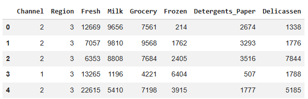
Here, we load the dataset using Pandas and display the first 5 rows to understand its structure, features and sample values.

Downlaod dataset from here

Python `

df = pd.read_csv("/content/Wholesale customers data.csv")

df.head()

`

**Output:

Dataset

Step 3: Explore Statistical Summary of the Data

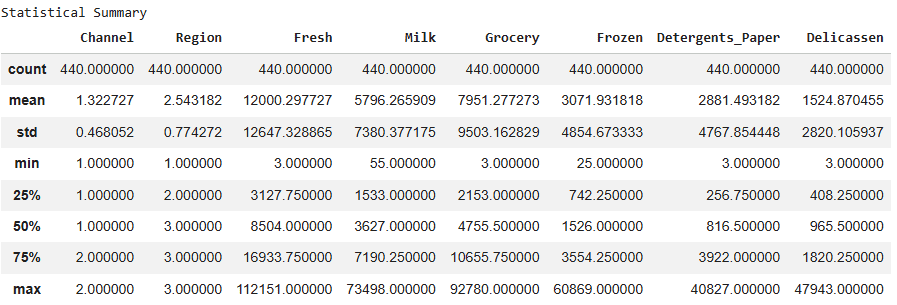
In this step, we use describe() to view key statistics of the dataset which helps in understanding data distribution and spotting anomalies.

Python `

print("\nStatistical Summary") display(df.describe())

`

**Output:

Statistical Summary

Step 4: Prepare Features and Target, Split Data

Here, we separate the dataset into features (X) and target labels (y), convert the target into binary format and split the data into training and testing sets for model training and evaluation.

Python `

X = df.drop('Channel', axis=1) y = df['Channel'].map({1:1, 2:0}) X_train, X_test, y_train, y_test = train_test_split( X, y, test_size=0.3, random_state=42 )

`

Step 5: Build and Train the XGBoost Model

Here we initialize the XGBoost classifier with specified hyperparameters, train it on the training data and make predictions on the test set.

• Defines the learning objective, tree depth, learning rate, number of trees and regularization to control overfitting.
• Fits the XGBoost model on the training data (X_train, y_train).
• Uses the trained model to predict target labels on the test set (X_test). Python `

params = { 'objective':'binary:logistic', 'max_depth':4, 'learning_rate':0.1, 'n_estimators':100, 'alpha':10 }

model = XGBClassifier(**params)

model.fit(X_train, y_train)

y_pred = model.predict(X_test)

`

Step 6: Evaluate Model Accuracy and Performance

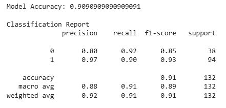
In this step, we measure how well the XGBoost model performs on the test set using accuracy and a detailed classification report.

Python `

accuracy = accuracy_score(y_test, y_pred) print("Model Accuracy:", accuracy)

print("\nClassification Report") print(classification_report(y_test, y_pred))

`

**Output:

Model evaluation

Step 7: Plot Confusion Matrix Heatmap

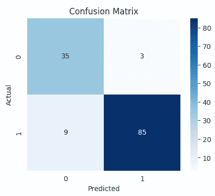
Visualizes the model’s confusion matrix using a heatmap, helping to quickly identify correct and incorrect predictions.

Python `

plt.figure(figsize=(5,4)) cm = confusion_matrix(y_test, y_pred) sns.heatmap(cm, annot=True, fmt='d', cmap='Blues') plt.title("Confusion Matrix") plt.xlabel("Predicted") plt.ylabel("Actual") plt.show()

`

**Output:

Confusion Matrix

Step 8: Plot Feature Importance

Here we visualize the importance of each feature in the XGBoost model to understand which variables contribute most to predictions.

Python `

plt.figure(figsize=(8,6)) xgb.plot_importance(model) plt.title("Feature Importance") plt.show()

`

**Output:

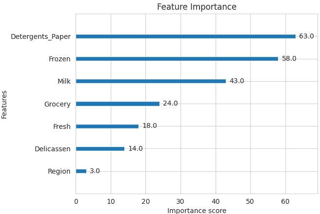
Feature Importance

Step 9: Visualize XGBoost Decision Tree

Plots one of the trained XGBoost decision trees to help understand how the model makes predictions based on feature splits.

Python `

plt.figure(figsize=(20,10)) xgb.plot_tree(model, num_trees=0) plt.show()

`

**Output:

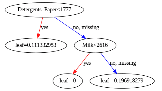
Decision Tree

Download code from here

Advantages

XGBoost includes several features and characteristics that make it useful in many scenarios:

• Scalable for large datasets with millions of records.
• Supports parallel processing and GPU acceleration.
• Offers customizable parameters and regularization for fine-tuning.
• Includes feature importance analysis for better insights.
• Available across multiple programming languages and widely used by data scientists.

Disadvantages

XGBoost also has certain aspects that require caution or consideration:

• Computationally intensive; may not be suitable for resource-limited systems.
• Sensitive to noise and outliers; careful preprocessing required.
• Can overfit, especially on small datasets or with too many trees.
• Limited interpretability compared to simpler models, which can be a concern in fields like healthcare or finance.