CART (Classification And Regression Tree) in Machine Learning (original) (raw)
Last Updated : 4 Dec, 2025
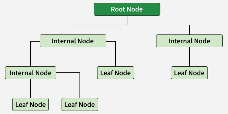
To break a dataset into smaller, meaningful groups, CART (Classification and Regression Tree) is used which builds a decision tree that predicts outcomes for both classification and regression tasks. It works by splitting data based on rules that reduce error at each step.
- Uses binary splits at every node.
- Simple to understand and interpret.
- Works for both numeric and categorical data.
- Forms the base of advanced models like Random Forest, Gradient Boosting and XGBoost.
How CART Builds a Decision Tree
CART (Classification and Regression Trees) constructs a decision tree by recursively splitting the dataset based on the feature and threshold that produce the highest reduction in impurity (for classification) or error (for regression)
CART
**Step 1: Evaluate Best Split for Each Feature
- Check all features and their possible split values.
- Compute impurity or error.
- Identify the split that gives the maximum reduction in impurity or error.
**Step 2: Select the Optimal Split
- Compare impurity decrease for all features.
- Choose the feature and threshold pair with the best score.
- This becomes the splitting rule for the current node.
**Step 3: Create Binary Child Nodes
- Split the dataset into Left Node (values less than or equal to threshold) and Right Node (values greater than or equal to threshold).
- Assign corresponding samples to each child node.
**Step 4: Apply Recursive Splitting
- Repeat the same process for each child node.
- Continue until a stopping condition is met.
CART for Classification
CART is used for classification tasks when the output variable is categorical.
**How it Works
- Recursively splits the dataset to increase class purity at each step.
- Uses Gini Impurity to select the best feature and threshold for splitting.
- Continues splitting until a stopping rule is met such as maximum tree depth or minimum required samples.
CART chooses splits that produce the purest possible child nodes.
CART for Regression
CART is used for regression tasks where the output variable is numerical.
**How it Works
- Splits the data to minimize residual error between actual and predicted values.
- Uses Mean Squared Error (MSE) or Residual Sum of Squares (RSS) as the splitting criterion.
- Each leaf node stores the mean of the target values within that node, which becomes the prediction for new samples.
This helps CART create a tree that provides the lowest possible prediction error.
Splitting Criteria in CART
CART uses different metrics to choose the best splitting rule depending on whether the problem is a classification or regression task. The goal is to find the split that produces the purest child nodes (for classification) or minimum prediction error (for regression).
Splitting Criteria for Classification
CART uses Gini Impurity to measure how mixed the classes are in a node.
Gini Impurity indicates how likely a randomly chosen sample from the node would be incorrectly classified if it were assigned labels according to class distribution.
\text{Gini} = 1 - \sum_{i=1}^{n} p_i^2
Where:
- p_i: proportion of class in i the node
- n: number of classes
- Gini = 0: Node is completely pure (only one class)
- Gini close to 1: Node contains a mix of many classes and is highly impure.
Splitting Criteria for Regression
For regression problems, CART uses Residual Sum of Squares (RSS) or Mean Squared Error (MSE) to find the best split.
**Residual Sum of Squares (RSS): RSS measures the total squared difference between actual output values and predicted values.
RSS = \sum (y - \hat{y})^2
Where:
- y: actual value
- \hat{y}: predicted value
**Mean Squared Error (MSE): MSE is simply RSS divided by the number of samples.
MSE = \frac{1}{n} \sum (y - \hat{y})^2
Lower RSS or MSE indicates a better split and CART selects the threshold that minimizes the prediction error in the resulting child nodes.
Pruning in CART
Pruning is used to prevent overfitting by trimming branches of the decision tree that add little or no improvement to model accuracy. It simplifies the tree, improves generalization and reduces model complexity.
**Types of Pruning in CART
- **Cost Complexity Pruning: Removes branches by comparing the trade off between tree accuracy and tree size, keeping only those nodes that significantly improve performance.
- **Reduced Error Pruning: Eliminates nodes that do not improve the model’s accuracy on a validation dataset, ensuring only beneficial splits remain.
Common Stopping or Pruning Criteria Used in CART
- **Maximum tree depth reached: The tree stops growing after a predefined maximum depth.
- **Minimum samples required to split a node: Splitting stops when a node has fewer samples than the minimum required.
- **No further improvement in impurity: If a split does not reduce impurity or error, CART stops splitting.
- **Node becomes pure: When all samples belong to one class, no further split is needed.
Hyperparameters in CART
CART provides several hyperparameters to control the tree structure, prevent overfitting and improve model performance. Important hyperparameters include:
- **max_depth: Controls the maximum depth of the tree, preventing it from growing too deep and overfitting the data.
- **min_samples_split: Specifies the minimum number of samples required to split an internal node; higher values make the tree more conservative.
- **min_samples_leaf: Determines the minimum number of samples allowed in a leaf node, helping avoid very small or unstable leaves.
- **max_features: Defines the number of features to consider while looking for the best split; useful for reducing computation and variance.
- **criterion: Specifies the function used to evaluate the split gini or entropy for classification and MSE for regression.
Step-By-Step Implementation
Here we builds and evaluates a Decision Tree (CART) model on the Iris dataset, generating predictions, accuracy metrics and visualizations of the trained tree using Matplotlib and Graphviz.
Step 1: Import Required Libraries
Here we will import pandas, seaborn, matplotlib and scikit learn.
Python `
import pandas as pd import seaborn as sns import matplotlib.pyplot as plt
from sklearn.datasets import load_iris from sklearn.model_selection import train_test_split from sklearn.tree import DecisionTreeClassifier, export_graphviz from sklearn.metrics import accuracy_score, confusion_matrix, classification_report from sklearn import tree
import pydotplus from IPython.display import Image
`
Step 2: Load and Prepare the Dataset
- Convert the dataset into a DataFrame for easier manipulation.
- Add the target variable species to the DataFrame.
- Separate feature matrix X and target vector y. Python `
iris = load_iris() df = pd.DataFrame(iris.data, columns=iris.feature_names) df['species'] = iris.target
X = iris.data y = iris.target
`
Step 3: Split Data into Training and Testing Sets
- We divide the dataset into training (80%) and testing (20%) using train_test_split.
- random_state ensures reproducibility.
- Training set is used to build the model; testing set evaluates performance. Python `
X_train, X_test, y_train, y_test = train_test_split( X, y, test_size=0.2, random_state=42)
`
Step 4: Train the Decision Tree
- We create a DecisionTreeClassifier, using entropy as the criterion.
- Entropy helps measure impurity for classification tasks.
- The model learns patterns from the training data using recursive binary splitting. Python `
model = DecisionTreeClassifier(criterion="entropy", random_state=42) model.fit(X_train, y_train)
`
Step 5: Make Predictions and Evaluate Model
- Predict the output for the test set using model.predict().
- Use a confusion matrix to visualize correct and incorrect predictions.
- sns.heatmap() creates a visual representation of the confusion matrix. Python `
y_pred = model.predict(X_test)
print("\nConfusion Matrix:") cm = confusion_matrix(y_test, y_pred) sns.heatmap(cm, annot=True, cmap="Blues", fmt="d") plt.title("Confusion Matrix") plt.xlabel("Predicted") plt.ylabel("Actual") plt.show()
`
**Output:
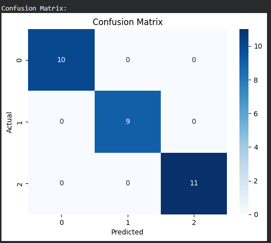
Confusion Matrix
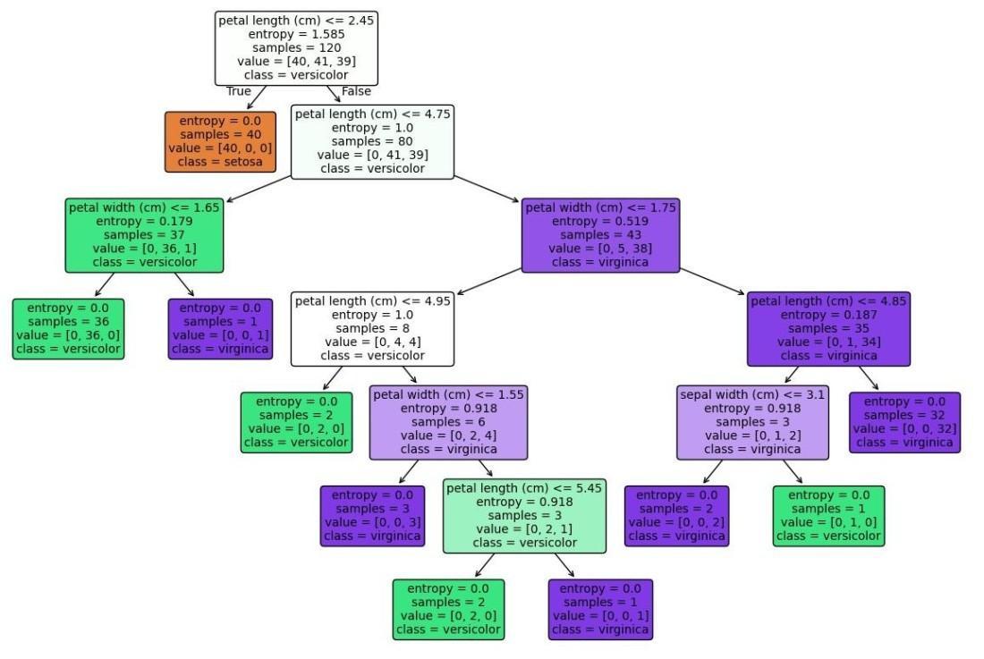
Step 6: Visualize the Decision Tree
- tree.plot_tree() plots the decision tree with node details.
- We display features, classes, node colors and structure.
- Helps understand how CART splits data at each level. Python `
plt.figure(figsize=(15,10)) tree.plot_tree( model, feature_names=iris.feature_names, class_names=iris.target_names, filled=True, rounded=True, fontsize=10 ) plt.show()
`
**Output:
You can download full code from here
Applications
- **Medical Diagnosis: Used to classify diseases based on symptoms, test results and patient history.
- **Blood Donor Classification: Helps predict whether a person is a suitable and safe blood donor.
- **Financial Risk Modeling: Assesses credit risk, loan default probability and fraud detection.
- **Customer Churn Prediction: Identifies customers likely to leave a service in telecom, banking or e-commerce.
- **Environmental Modelling: Used for predicting pollution levels, weather patterns and ecological changes.
- **Image and Pattern Recognition: Helps classify objects, detect patterns and recognize visual features.
Advantages
- The tree structure is very easy to understand and interpret, making decision-making transparent and human-readable.
- CART handles both regression and classification tasks, supporting numerical as well as categorical targets.
- It makes no assumptions about data distribution and works well even without linearity or normality.
- It automatically performs feature selection by choosing only the most important splitting features.
- It handles non-linear relationships effectively by capturing complex patterns through hierarchical splits.
Limitations
- CART is prone to overfitting, especially when the tree grows too deep.
- It has high variance, meaning small changes in the data can lead to very different tree structures.
- The model is sensitive to minor data variations, which can significantly alter the split decisions.
- CART performs only binary splits, which may not always be optimal for certain types of datasets.