Continuous Probability Distributions for Machine Learning (original) (raw)

Last Updated : 23 Jul, 2025

In machine learning, we often face uncertainty in our data. Continuous probability distributions help us understand this uncertainty by showing how likely different values are to occur. Whether predicting prices or classifying images, these distributions let us make smarter, more reliable predictions by accounting for the randomness in the real world.

**Continuous Probability Distributions

A probability distribution is a mathematical function that describes the likelihood of different outcomes for a random variable. Continuous probability distributions (CPDs) are probability distributions that apply to continuous random variables. It describes events that can take on any value within a specific range, like the height of a person or the amount of time it takes to complete a task.

In continuous probability distributions, two key functions describe the likelihood of a variable taking on specific values:

**1. Probability Density Function (PDF): The probability density function gives the probability density at a specific point or interval for a continuous random variable. It indicates how likely the variable is to fall within a small interval around a particular value.

The height of the PDF curve at any point represents the probability density at that value.
Higher density implies a higher probability of the variable taking on values around that point.

**2. Cumulative Distribution Function (CDF): The Cumulative Distribution Function gives the probability that a random variable is less than or equal to a specific value.It provides a cumulative view of the probability distribution, starting at 0 and increasing to 1 as the value of the random variable increases.

The CDF starts at 0 for the smallest possible value of the random variable (since there is no probability below this value) and approaches 1 as the value approaches infinity (since the probability of the variable being less than or equal to infinity is 1).

CDF is the integral of the PDF and the PDF is the derivative of the CDF.

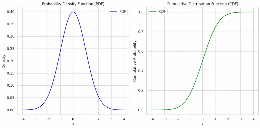
Visual-Difference-between-PDF-and-CDF

Visual Difference between CDF & PDF in Continuous Probability Distributions

**Importance of Continuous Probability Distribution

**Modeling Uncertainty: They help represent uncertainty in predictions, allowing probabilistic outputs instead of fixed values.
**Gaussian Distribution: Widely used in models like regression and Bayesian networks for error modeling and assumption of normality.
**Maximum Likelihood Estimation (MLE): Many algorithms rely on continuous distributions to estimate model parameters that maximize the likelihood of observed data.
**Bayesian Inference: Continuous distributions are essential in Bayesian models to update beliefs about parameters based on new data.
**Generative Models: Models like Gaussian Mixture Models and Variational Autoencoders use continuous distributions to learn and generate data.

Types of Continuous Probability Distributions

1. Normal Distribution (Bell Curve) or Gaussian Distribution

The Gaussian Distribution is a bell-shaped, symmetrical basic continuous probability distribution. Two factors define it:

the standard deviation (σ), which indicates the distribution's spread or dispersion,
the mean (μ), which establishes the distribution.

For a random variable x, it is expressed as,

f(x) =\frac{1}{\sqrt{2 \pi \sigma^2}} \exp \left( -\frac{1}{2} \left( \frac{x - \mu}{\sigma} \right)^2 \right)

Normal-Distribution

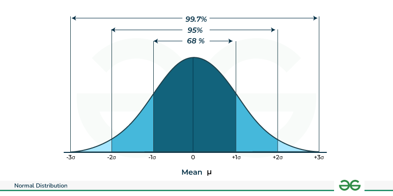
Note: The shape of the Normal Distribution is such that about 68% of the values fall within one standard deviation of the mean (μ ± σ), about 95% fall within two standard deviations (μ ± 2σ) and about 99.7% fall within three standard deviations (μ ± 3σ).

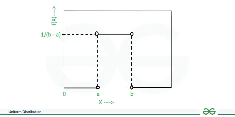
**Uniform Distribution

The Uniform Distribution is a continuous probability distribution where all values within a specified range are equally likely to occur.

Parameters: Lower bound (a) and upper bound (b).
The mean of a uniform distribution is \mu = \frac{a + b}{2}and the variance is \sigma^2 = \frac{(b - a)^2}{12}

It is expressed as:

f(x) = \frac{1}{b - a} \quad \text{for } a \leq x \leq b

Uniform-Distribution

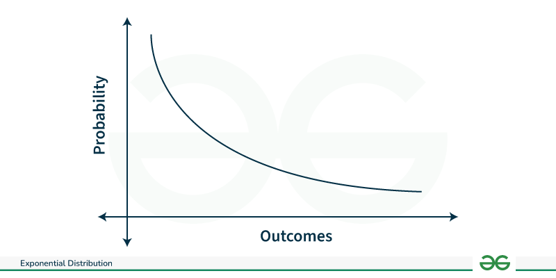
**Exponential Distribution

The exponential distribution is a continuous probability distribution that represents the duration between occurrences in a Poisson process, which occurs continuously and independently at a constant average rate.

Parameter: Rate parameter (λ).
The mean of the exponential distribution is 1/_λ and the variance is 1/λ^2.

For a random variable x, it is expressed as

f(x) = \lambda e^{-\lambda x} \quad \text{for } x \geq 0

Exponential-Distribution

**Chi-Squared Distribution

The Chi-Squared Distribution is a continuous probability distribution that arises in statistics, particularly in hypothesis testing and confidence interval estimation.

It is characterized by a single parameter, often denoted as _k ,which represents the degrees of freedom.
The mean of the Chi-Squared Distribution is k and the variance is 2__k.

For a random variable x, it is expressed as

f(x) = \frac{1}{2^{k/2} \Gamma(k/2)} \left( \frac{x}{2} \right)^{k/2 - 1} e^{-x/2}

Chi-Squared-Distribution-(1)

Determining the distribution of a variable

**Example : Lets understand the distribution of a variable with the help of iris dataset .

Python `

import pandas as pd import numpy as np import matplotlib.pyplot as plt from scipy.stats import norm

url = "https://raw.githubusercontent.com/uiuc-cse/data-fa14/gh-pages/data/iris.csv" iris_data = pd.read_csv(url)

selected_feature = 'petal_length' selected_data = iris_data[selected_feature]

plt.figure(figsize=(12, 5)) plt.subplot(1, 2, 1) plt.hist(selected_data, bins=30, density=True, color='skyblue', alpha=0.6) plt.title('Histogram of {}'.format(selected_feature)) plt.xlabel(selected_feature) plt.ylabel('Density') plt.grid(True)

estimated_mean, estimated_std = np.mean(selected_data), np.std(selected_data)

plt.subplot(1, 2, 2) plt.hist(selected_data, bins=30, density=True, color='skyblue', alpha=0.6)

x = np.linspace(np.min(selected_data), np.max(selected_data), 100) pdf = norm.pdf(x, estimated_mean, estimated_std) plt.plot(x, pdf, color='red', linestyle='--', linewidth=2)

plt.title('Histogram and Fitted Gaussian Distribution of {}'.format( selected_feature)) plt.xlabel(selected_feature) plt.ylabel('Density') plt.legend(['Fitted Gaussian Distribution', 'Histogram']) plt.grid(True)

plt.tight_layout() plt.show()

**Output:

download

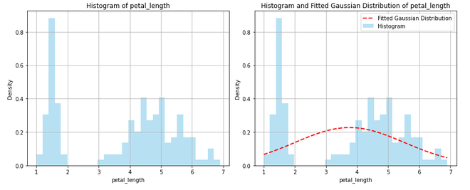
**Histogram of Petal Length: It shows the frequency distribution of the 'petal_length' feature from the Iris dataset.
**Histogram with Fitted Gaussian Curve: This combines the same histogram with a red dashed line representing the fitted normal distribution (Gaussian) based on the mean and standard deviation of the data.

Continuous Probability Distributions for Machine Learning (original) (raw)