Denoising AutoEncoders In Machine Learning (original) (raw)

Last Updated : 7 Aug, 2025

Autoencoders are neural networks for unsupervised learning that compress input data into a low-dimensional space (using an encoder) and then reconstruct it (using a decoder), training the network to minimize the reconstruction error between the original input and its reconstructed output. If the hidden layer is too large, autoencoders may simply learn to replicate the input perfectly, functioning as an identity mapping and failing to extract meaningful features.

• Denoising autoencoders address this by providing a deliberately noisy or corrupted version of the input to the encoder, but still using the original, clean input for calculating loss.
• This trains the model to learn useful, robust features and reduces the chance of simply replicating the input.

Architecture of DAE

The denoising autoencoder (DAE) architecture resembles a standard autoencoder and consists of two main components:

Encoder

• A neural network (one or more layers) that transforms noisy input data into a lower-dimensional encoding.
• Noise can be introduced by adding Gaussian noise or randomly masking/missing some inputs.

Decoder

• A neural network (one or more layers) that reconstructs the original data from the encoding.
• The loss is calculated between the decoder’s output and the original clean input, not the noisy one.

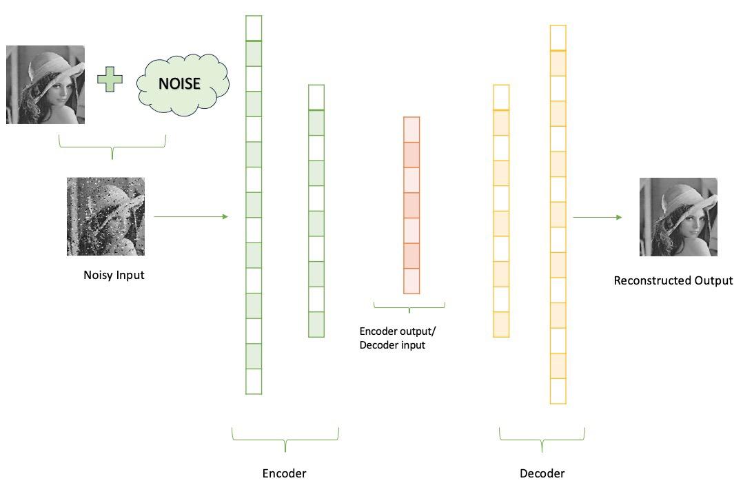
DAE architecture

Step-by-Step Implementation of DAE

Let's implement DAE in PyTorch for MNIST dataset.

Step 1: Import Libraries

Lets import the necessary libraries,

• **torch: Core PyTorch library for deep learning.
• **torch.utils.data: For handling custom datasets and loaders.
• **torch.nn: Provides modules for building neural networks, such as layers and activations.
• **torch.optim: Contains optimization algorithms, like Adam.
• **torchvision.datasets: Includes popular computer vision datasets, such as MNIST.
• **torchvision.transforms: For preprocessing transforms (e.g., normalization, tensor conversion).
• **matplotlib.pyplot: Matplotlib pyplot is used for data and result visualization.
• Set up the device to use GPU if available otherwise CPU. Python `

import torch import torch.utils.data from torchvision import datasets, transforms import numpy as np import pandas as pd from torch import nn, optim

device = 'cuda' if torch.cuda.is_available() else 'cpu'

`

Step 2: Load the Dataset and Define Dataloader

We prepare the MNIST handwritten digits dataset:

• **transforms.Compose: Creates a pipeline of transformations.
• **ToTensor(): Converts PIL Images or numpy arrays to PyTorch tensors.
• **Normalize(0, 1): (For MNIST, actually not changing the scale, but prepares the tensor for potential mean/variance normalization.)
• **datasets.MNIST: Downloads and loads the MNIST dataset for training and testing.
• **DataLoader: Enables efficient batch processing and optional shuffling during training. Python `

transform = transforms.Compose([ transforms.ToTensor(), transforms.Normalize(0, 1) ])

mnist_dataset_train = datasets.MNIST( root='./data', train=True, download=True, transform=transform) mnist_dataset_test = datasets.MNIST( root='./data', train=False, download=True, transform=transform)

batch_size = 128

train_loader = torch.utils.data.DataLoader( mnist_dataset_train, batch_size=batch_size, shuffle=True) test_loader = torch.utils.data.DataLoader( mnist_dataset_test, batch_size=5, shuffle=False)

`

Step 3: Define Denoising Autoencoder(DAE) Model

We design a neural network with an encoder and decoder:

• **Encoder: Three fully connected layers reduce the input (flattened image) from 784 dimensions down to 128.
• **Decoder: Three layers expand the compressed encoding back to 784.
• **nn.Linear: A fully connected neural network layer that applies a linear transformation to input data.
• **nn.ReLU: The Rectified Linear Unit activation function that replaces negative values with zero.
• **nn.Sigmoid: The Sigmoid activation function that squashes values to the range (0, 1).
• **self.relu: An instance of nn.ReLU used to apply the ReLU activation function to layer outputs.
• **self.sigmoid: An instance of nn.Sigmoid used to apply the Sigmoid activation to layer outputs. Python `

class DAE(nn.Module): def init(self): super().init() self.fc1 = nn.Linear(784, 512) self.fc2 = nn.Linear(512, 256) self.fc3 = nn.Linear(256, 128) self.fc4 = nn.Linear(128, 256) self.fc5 = nn.Linear(256, 512) self.fc6 = nn.Linear(512, 784) self.relu = nn.ReLU() self.sigmoid = nn.Sigmoid()

def encode(self, x):
    h1 = self.relu(self.fc1(x))
    h2 = self.relu(self.fc2(h1))
    return self.relu(self.fc3(h2))

def decode(self, z):
    h4 = self.relu(self.fc4(z))
    h5 = self.relu(self.fc5(h4))
    return self.sigmoid(self.fc6(h5))

def forward(self, x):
    q = self.encode(x.view(-1, 784))
    return self.decode(q)

`

Step 4: Define the Training Function

We define the Training function in which:

• For each batch, add Gaussian noise to simulate corruption.
• Forward the noisy batch through the model.
• Compute the loss using Mean Squared Error between the output and original.
• Perform backpropagation and optimize weights.
• Print progress and average epoch loss. Python `

def train(epoch, model, train_loader, optimizer, cuda=True): model.train() train_loss = 0 for batch_idx, (data, _) in enumerate(train_loader): data = data.to(device) optimizer.zero_grad() data_noise = torch.randn(data.shape).to(device) data_noise = data + data_noise recon_batch = model(data_noise) loss = criterion(recon_batch, data.view(data.size(0), -1)) loss.backward() train_loss += loss.item() * len(data) optimizer.step() if batch_idx % 100 == 0: print('Train Epoch: {} [{}/{} ({:.0f}%)]\tLoss: {:.6f}'.format( epoch, batch_idx * len(data), len(train_loader.dataset), 100. * batch_idx / len(train_loader), loss.item())) print('====> Epoch: {} Average loss: {:.4f}'.format( epoch, train_loss / len(train_loader.dataset)))

`

Step 5: Initialize Model, Optimizer and Loss Function

We need to initialize the model along with the optimizer and Loss Function,

• Instantiate the DAE model and move to the selected device.
• Use Adam optimizer with learning rate 0.01.
• Set reconstruction loss to Mean Squared Error. Python `

epochs = 10 model = DAE().to(device) optimizer = optim.Adam(model.parameters(), lr=1e-2) criterion = nn.MSELoss()

`

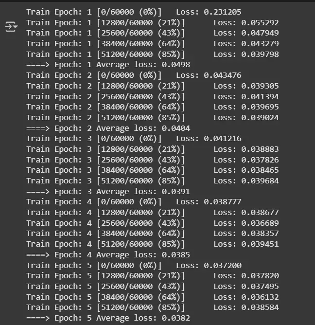
Step 6: Train the Model

Loop over the dataset for the given number of epochs, invoking the training function.

Python `

for epoch in range(1, epochs + 1): train(epoch, model, train_loader, optimizer, True)

`

**Output:

Testing Phase

Step 7: Evaluate and Visualize the Model

We evaluate the predictions of the model and also visualize the results,

• Take a small batch from the test set.
• Add noise and reconstruct using the trained autoencoder.
• Plot noisy, reconstructed and original images side by side. Python `

import matplotlib.pyplot as plt

for batch_idx, (data, labels) in enumerate(test_loader): data = data.to(device) optimizer.zero_grad() data_noise = torch.randn(data.shape).to(device) data_noise = data + data_noise recon_batch = model(data_noise) break

plt.figure(figsize=(20, 12)) for i in range(5): print(f" Image {i} with label {labels[i]}", end="") plt.subplot(3, 5, 1 + i) plt.imshow(data_noise[i, :, :, :].view( 28, 28).cpu().detach().numpy(), cmap='binary') plt.axis('off') plt.subplot(3, 5, 6 + i) plt.imshow(recon_batch[i, :].view( 28, 28).cpu().detach().numpy(), cmap='binary') plt.axis('off') plt.subplot(3, 5, 11 + i) plt.imshow(data[i, :, :, :].view( 28, 28).cpu().detach().numpy(), cmap='binary') plt.axis('off') plt.show()

`

**Output:

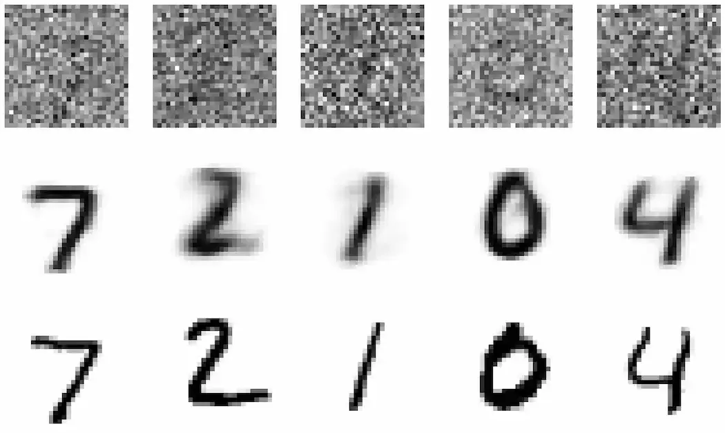
Result

**Row 1: Noisy images (input)
**Row 2: Denoised outputs (autoencoder reconstructions)
**Row 3: Original images (target, uncorrupted)

Applications of DAE

• **Image Denoising: Removing noise from images to restore clear, high-quality visuals.
• **Data Imputation: Filling in missing values or reconstructing incomplete data entries.
• **Feature Extraction: Learning robust features that improve performance for tasks like classification and clustering.
• **Anomaly Detection: Identifying outliers by measuring reconstruction errors on new data.
• **Signal and Audio Denoising: Cleaning noisy sensor or audio signals, such as in speech or biomedical recordings.

**Advantages

• Help models learn robust, meaningful features that are less sensitive to noise or missing data.
• Reduce the risk of merely copying input data (identity mapping), especially when compared to basic autoencoders.
• Improve performance on tasks such as image denoising, data imputation and anomaly detection by reconstructing clean signals from corrupted inputs.
• Enhance the generalizability of learned representations, making models more useful for downstream tasks.

**Limitations

• May require careful tuning of the type and level of noise added to the inputs for optimal performance.
• Can be less effective if the noise model used during training does not match the type of corruption seen in real-world data.
• High computational cost, especially with large datasets or deep architectures.
• Like other unsupervised methods, provide no guarantees that learned features will be directly useful for specific downstream supervised tasks.