Different Variants of Gradient Descent (original) (raw)
Last Updated : 29 Sep, 2025
Gradient descent is a optimization algorithm in machine learning used to minimize functions by iteratively moving towards the minimum. It's important as fine-tuning parameters helps us to reduce prediction errors. In this article we are going to explore different variants of gradient descent algorithms.
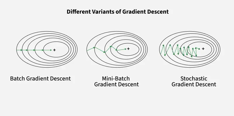
Different Variants of Gradient Descent
1. Batch Gradient Descent
Batch Gradient Descent is a variant of the gradient descent algorithm where the entire dataset is used to compute the gradient of the loss function with respect to the parameters. In each iteration the algorithm calculates the average gradient of the loss function for all the training examples and updates the model parameters accordingly.
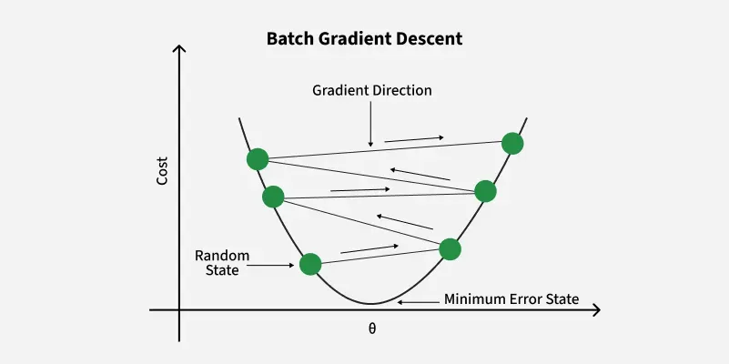
Batch Gradient Descent
The update rule for batch gradient descent is:
\theta = \theta - \eta \nabla J(\theta)
where:
- \theta represents the parameters of the model
- \eta is the learning rate
- ∇J(θ) is the gradient of the loss function J(θ)) with respect to θ.
Python Implementation
- Computes the gradient using all training examples.
- Averages the gradient over the full dataset.
- Updates theta once per epoch.
- Suitable for small to medium datasets. Python `
def batch_gradient_descent(X, y, theta, lr=0.01, epochs=100): m = len(y) for _ in range(epochs): gradients = (1 / m) * X.T @ (X @ theta - y) theta -= lr * gradients return theta
`
**Advantages
- **Stable Convergence: Since the gradient is averaged over all training examples the updates are less noisy and more stable.
- **Global View: It considers the entire dataset for each update providing a global perspective of the loss landscape.
**Disadvantages
- **Computationally Expensive: It Processing the entire dataset in each iteration can be slow and resource-intensive especially for large datasets.
- **Memory Intensive: This requires storing and processing the entire dataset in memory which can be impractical for very large datasets.
2. Stochastic Gradient Descent
Stochastic Gradient Descent (SGD) is a variant of the gradient descent algorithm where the model parameters are updated using the gradient of the loss function with respect to a single training example at each iteration. Unlike batch gradient descent which uses the entire dataset SGD updates the parameters more frequently, leading to faster convergence.
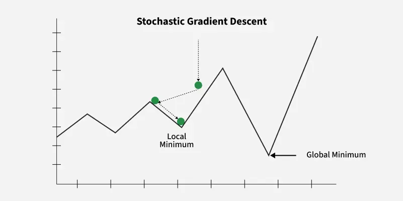
Stochastic Gradient Descent
The update rule for SGD is:
\theta = \theta - \eta \nabla J(\theta; x^{(i)}, y^{(i)})
where:
- θ represents the parameters of the model,
- η is the learning rate,
- \nabla J(\theta; x^{(i)}, y^{(i)}) is the gradient of the loss function J(θ) with respect to θ for the i^{th} training example (x^{(i)}, y^{(i)}).
Python Implementation
- Updates theta using one example at a time.
- Leads to faster but noisier updates.
- Useful for online learning and large datasets.
- More sensitive to learning rate. Python `
import numpy as np
def stochastic_gradient_descent(X, y, theta, lr=0.01, epochs=100): m = len(y) for _ in range(epochs): for i in range(m): xi = X[i:i + 1] yi = y[i:i + 1] gradient = xi.T @ (xi @ theta - yi) theta -= lr * gradient return theta
`
**Advantages
- **Faster Convergence: Frequent updates can lead to faster convergence, especially in large datasets.
- **Less Memory Intensive: Since it processes one training example at a time, it requires less memory compared to batch gradient descent.
- **Better for Online Learning: Suitable for scenarios where data comes in a stream, allowing the model to be updated continuously.
**Disadvantages
- **Noisy Updates: Updates can be noisy, leading to a more erratic convergence path.
- **Potential for Overshooting: The frequent updates can cause the algorithm to overshoot the minimum, especially with a high learning rate.
- **Hyperparameter Sensitivity: Requires careful tuning of the learning rate to ensure stable and efficient convergence.
3. Mini-Batch Gradient Descent
Mini-Batch Gradient Descent is a compromise between Batch Gradient Descent and Stochastic Gradient Descent. Instead of using the entire dataset or a single training example Mini-Batch Gradient Descent updates the model parameters using a small, random subset of the training data called a mini-batch.
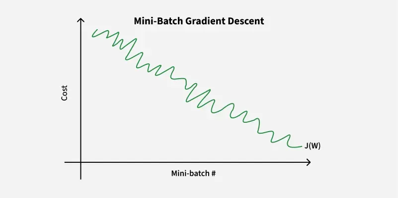
Mini-Batch Gradient Descent
Update rule for Mini-Batch Gradient Descent is:
\theta = \theta - \eta \nabla J(\theta; \{x^{(i)}, y^{(i)}\}_{i=1}^m)
where:
- θ represents the parameters of the model,
- η is the learning rate,
- \{x^{(i)}, y^{(i)}\}_{i=1}^{m}represents a mini-batch of mmm training examples,
- \nabla J(\theta; \{x^{(i)}, y^{(i)}\}_{i=1}^m) is the gradient of the loss function J(\theta) with respect to θ for the mini-batch.
Python Implementation
- Splits data into mini-batches like 32 samples.
- Shuffles data for better generalization.
- Combines speed of SGD with stability of Batch GD.
- Supports parallel computation like GPUs. Python `
def mini_batch_gradient_descent(X, y, theta, lr=0.01, epochs=100, batch_size=32): m = len(y) for _ in range(epochs): indices = np.random.permutation(m) X_shuffled, y_shuffled = X[indices], y[indices] for i in range(0, m, batch_size): xb = X_shuffled[i:i + batch_size] yb = y_shuffled[i:i + batch_size] gradient = (1 / len(yb)) * xb.T @ (xb @ theta - yb) theta -= lr * gradient return theta
`
**Advantages
- **Faster Convergence: By using mini-batches, it achieves a balance between the noisy updates of SGD and the stable updates of Batch Gradient Descent, often leading to faster convergence.
- **Reduced Memory Usage: Requires less memory than Batch Gradient Descent as it only needs to store a mini-batch at a time.
- **Efficient Computation: Allows for efficient use of hardware optimizations and parallel processing, making it suitable for large datasets.
**Disadvantages
- **Complexity in Tuning: Requires careful tuning of the mini-batch size and learning rate to ensure optimal performance.
- **Less Stable than Batch GD: While more stable than SGD, it can still be less stable than Batch Gradient Descent, especially if the mini-batch size is too small.
- **Potential for Suboptimal Mini-Batch Sizes: Selecting an inappropriate mini-batch size can lead to suboptimal performance and convergence issues.
Momentum-Based Gradient Descent
Momentum-Based Gradient Descent is an enhancement of standard gradient descent algorithm that aims to accelerate convergence particularly in the presence of high curvature, small but consistent gradients or noisy gradients. It introduces a velocity term that accumulates the gradient of the loss function over time thereby smoothing the path taken by the parameters.
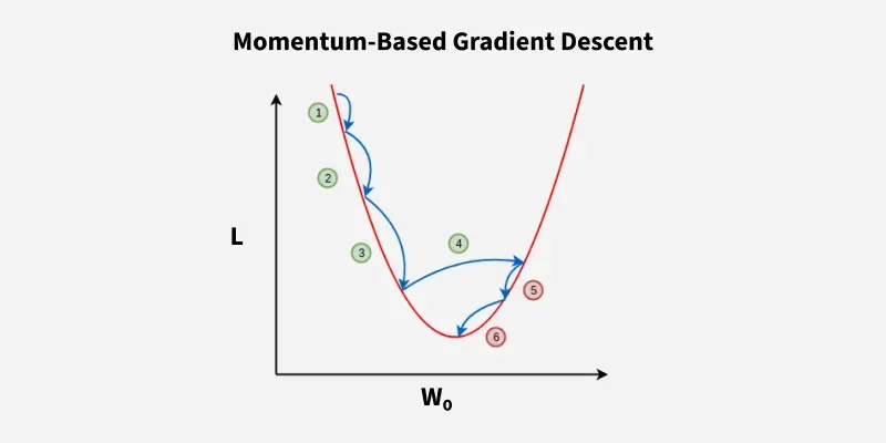
Momentum-Based Gradient Descent
The update rule for Momentum-Based Gradient Descent is:
v_t = \gamma v_{t-1} + \eta \nabla J(\theta_t)
\theta_{t+1} = \theta_t - v_t
where:
- v_t is the velocity at iteration t,
- \gamma is the momentum term (typically between 0 and 1),
- \etais the learning rate,
- \nabla J(\theta_t) is the gradient of the loss function J(θ) with respect to θ at iteration t.
Python Implementation
- Maintains a velocity vector v to smooth updates.
- gamma controls how much past gradients influence current step.
- Helps in faster convergence especially in noisy loss surfaces.
- Common in deep learning frameworks like TensorFlow and PyTorch. Python `
def momentum_gradient_descent(X, y, theta, lr=0.01, epochs=100, gamma=0.9): m = len(y) v = np.zeros_like(theta) for _ in range(epochs): gradient = (1 / m) * X.T @ (X @ theta - y) v = gamma * v + lr * gradient theta -= v return theta
`
**Advantages
- **Accelerated Convergence: Helps in faster convergence especially in scenarios with small but consistent gradients.
- **Smoother Updates: Reduces the oscillations in the gradient updates, leading to a smoother and more stable convergence path.
- **Effective in Ravines: Particularly effective in dealing with ravines or regions of steep curvature and is common in deep learning loss landscapes.
**Disadvantages
- **Additional Hyperparameter: Introduces an additional hyperparameter (momentum term) that needs to be tuned.
- **Complex Implementation: Slightly more complex to implement compared to standard gradient descent.
- **Potential Overcorrection: If not properly tuned the momentum can lead to overcorrection and instability in the updates.
Comparison between the variants of Gradient Descent
| **Variant | **Data Used | **Convergence | **Memory Usage | **Efficiency | **Key Advantage |
|---|---|---|---|---|---|
| **Batch Gradient Descent | Entire dataset | Stable but slow | High (entire dataset) | Computationally expensive | Stable convergence, global view of data |
| **Stochastic Gradient Descent | One example per iteration | Fast but noisy | Low (one example) | Less efficient | Faster convergence, good for online learning |
| **Mini-Batch Gradient Descent | Mini-batch of data | Faster and smoother | Medium (mini-batch) | Efficient, parallelizable | Balance of speed and stability |
| **Momentum-Based Gradient Descent | Entire dataset or mini-batch | Faster and smoother | Medium (like Mini-Batch) | Efficient with momentum | Accelerated convergence, smooth updates |