Gaussian Mixture Model (original) (raw)
Last Updated : 2 May, 2026
Gaussian Mixture Model (GMM) is a probabilistic clustering technique that models data as a combination of multiple Gaussian distributions, allowing more flexible grouping of data points.
- Assigns each data point a probability of belonging to different clusters
- Can handle overlapping clusters effectively
- Uses mean and covariance to define cluster shape
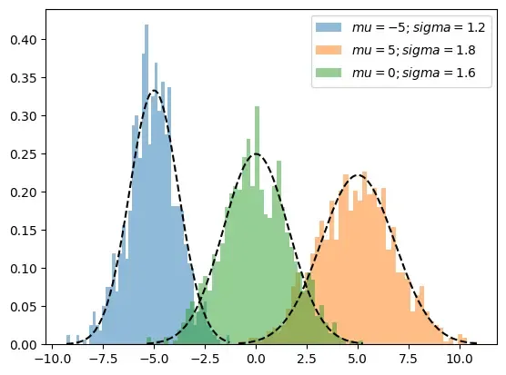
Visualization of three distinct one-dimensional Gaussian distributions
The above shown graph shows a three one-dimensional Gaussian distributions with distinct means and variances. Each curve represents the theoretical probability density function (PDF) of a normal distribution, highlighting differences in location and spread.
Working of GMM
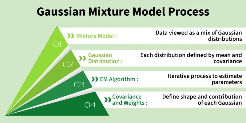
Working of Gaussian Mixture Model
A Gaussian Mixture Model assumes that the data is generated from a mixture of K Gaussian distributions, each representing a cluster. Every Gaussian has its own mean \mu_k, covariance \Sigma_k and mixing weight \pi_k.
1. Posterior Probability (Cluster Responsibility)
For a given data point xn, the probability that it belongs to cluster k:
P(z_n = k \mid x_n) = \frac{\pi_k \cdot \mathcal{N}(x_n \mid \mu_k, \Sigma_k)}{\sum_{j=1}^{K} \pi_j \cdot \mathcal{N}(x_n \mid \mu_j, \Sigma_j)}
**where:
- z_n is a latent variable indicating cluster assignment
- \pi_k is the mixing probability of the k-th Gaussian.
- \mathcal{N}(x_n \mid \mu_k, \Sigma_k)is the Gaussian distribution with mean \mu_k and covariance \Sigma_k
**2. Likelihood of a Data Point
The total likelihood of observing xnx_nxn under all Gaussians is:
P(x_n) = \sum_{k=1}^{K} \pi_k \cdot \mathcal{N}(x_n \mid \mu_k, \Sigma_k)
This represents how well the mixture as a whole explains the data point.
3. Expectation-Maximization (EM) Algorithm
GMM parameters are estimated using the EM algorithm:
**E-step (Expectation): Compute the responsibility of each cluster for every data point using current parameter values.
**M-step (Maximization): Update
- Means \mu_k
- Covariances \Sigma_k
- Mixing coefficients using the responsibilities from the E-step. The process continues until the model's log-likelihood stabilizes.
4. Log-Likelihood of the Mixture Model
The objective optimized by EM is:
L(\mu, \Sigma, \pi) = \prod_{n=1}^{N} \sum_{k=1}^{K} \pi_k \cdot \mathcal{N}(x_n \mid \mu_k, \Sigma_k)
EM increases this likelihood in every iteration.
Cluster Shapes in GMM
In GMM, each cluster is a Gaussian defined by:
- **Mean (μ): Center of the cluster.
- **Covariance (Σ): Controls the shape, orientation and spread of the cluster.
Because covariance matrices allow elliptical shapes, GMM can model:
- elongated clusters
- tilted clusters
- overlapping clusters
This makes GMM more flexible than methods like K-Means, which assumes only spherical clusters.
**Visualizing GMM often involves:
- Scatter plots showing raw data
- Elliptical contours (or KDE curves) showing the shape of each Gaussian component
These illustrate how GMM adapts to complex, real-world data distributions.
Implementing Gaussian Mixture Model (GMM)
Import required libraries. make_blobs creates a simple synthetic dataset for demo.
Python `
import numpy as np import matplotlib.pyplot as plt from sklearn.mixture import GaussianMixture from sklearn.datasets import make_blobs
`
Step 1: Generate synthetic data
creates 500 points in 2D grouped around 3 centers. cluster_std controls how tight or spread each cluster is. y is the true label (only for reference).
Python `
X, y = make_blobs( n_samples=500, centers=3, random_state=42, cluster_std=[1.0, 1.5, 0.8] # spread for each cluster )
`
Step 2: Fit the Gaussian Mixture Model
- fit(X) runs the EM algorithm to learn means, covariances and mixing weights.
- labels gives the cluster index for each point (the component with highest posterior probability). Python `
gmm = GaussianMixture( n_components=3, # number of Gaussian components covariance_type='full', random_state=42 )
gmm.fit(X)
labels = gmm.predict(X)
`
Step 3: Plot clusters and component centers
Points colored by assigned cluster and red X marks showing the learned Gaussian centers.
Python `
plt.figure(figsize=(8, 6))
scatter points colored by hard labels
plt.scatter(X[:, 0], X[:, 1], c=labels, cmap='viridis', s=50, edgecolor='k')
plot Gaussian centers
plt.scatter( gmm.means_[:, 0], gmm.means_[:, 1], s=300, c='red', marker='X', label='Centers' )
plt.title("Gaussian Mixture Model Clustering") plt.xlabel("Feature 1") plt.ylabel("Feature 2") plt.grid(True) plt.legend() plt.show()
`
**Output:
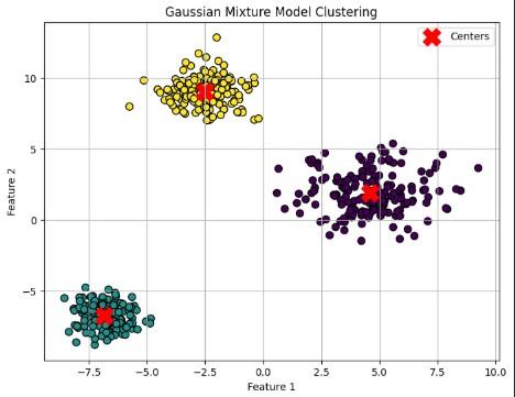
Plot clusters and component centers
You can download the complete code from here.
Use-Cases
- **Clustering: Discover underlying groups or structure in data (marketing, medicine, genetics).
- **Anomaly Detection: Identify outliers or rare events (fraud, medical errors).
- **Image Segmentation: Separate images into meaningful regions (medical, remote sensing).
- **Density Estimation: Model complex probability distributions for generative modeling.
Advantages
- **Flexible Cluster Shapes: Models ellipsoidal and overlapping clusters.
- **Soft Assignments: Assigns probabilistic cluster membership instead of hard labels.
- **Handles Missing Data: Robust to incomplete observations.
- **Interpretable Parameters: Each Gaussian’s mean, covariance and weight are easy to interpret.
Limitations
- **Initialization Sensitive: Results depend on starting parameter values can get stuck in local optima.
- **Computation Intensive: Slow for high-dimensional or very large datasets.
- **Assumes Gaussian Distributions: Not suitable for non-Gaussian cluster shapes.
- **Requires Cluster Number: Must specify the number of components/clusters before fitting.