Gaussian Naive Bayes (original) (raw)
Last Updated : 2 May, 2026
Gaussian Naive Bayes is a type of Naive Bayes method working on continuous attributes and the data features that follows Gaussian distribution throughout the dataset. This “naive” assumption simplifies calculations and makes the model fast and efficient.
- It is widely used because it performs well even with small datasets and is easy to implement and interpret.
- Works well with continuous numerical features
- Fast, simple, and effective for classification problems
- Commonly used in spam detection, medical diagnosis, and pattern recognition
Mathematics
Gaussian Naive Bayes
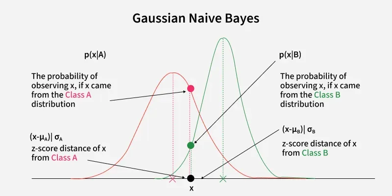
Gaussian Naive Bayes assumes that the likelihood (P(x_i|y)) follows the Gaussian Distribution for each x_i within y_k. Therefore,
P(x_i|y) = \frac{1}{\sigma \sqrt{2\pi}} e^{-\frac{(x - \mu)^2}{2\sigma^2}}
Where:
- x_i is the feature value,
- \mu is the mean of the feature values for a given class y_k,
- \sigma is the standard deviation of the feature values for that class,
- \pi is a constant (approximately 3.14159),
- e is the base of the natural logarithm.
To classify each new data point x the algorithm finds out the maximum value of the posterior probability of each class and assigns the data point to that class.
Why Gaussian Naive Bayes Works Well for Continuous Data?
Gaussian Naive Bayes is effective for continuous data because it assumes each feature follows a Gaussian (normal) distribution. When this assumption holds true the algorithm performs well. For example, in tasks like medical diagnosis or predicting house prices, where features such as age, income or measurements follow a normal distribution, Gaussian Naive Bayes can make accurate predictions.
Practical Example
To understand how Gaussian Naive Bayes works here's a simple binary classification problem using one feature: petal length.
| Petal Length (cm) | Class Label |
|---|---|
| 1.4 | 0 (Iris-setosa) |
| 1.3 | 0 (Iris-setosa) |
| 1.5 | 0 (Iris-setosa) |
| 4.5 | 1 (Iris-versicolor) |
| 4.7 | 1 (Iris-versicolor) |
| 4.6 | 1 (Iris-versicolor) |
We want to classify a new sample with **petal length = 1.6 cm.
**1. Separate by Class
- Class 0: [1.4, 1.3, 1.5]
- Class 1: [4.5, 4.7, 4.6]
**2. Calculate Mean and Variance
**For class 0:
- \mu_0 = \frac{1.4 + 1.3 + 1.5}{3} = 1.4
- \sigma_0^2 = \frac{(1.4 - 1.4)^2 + (1.3 - 1.4)^2 + (1.5 - 1.4)^2}{3} = 0.0067
**For class 1:
- \mu_1 = \frac{4.5 + 4.7 + 4.6}{3} = 4.6
- \sigma_1^2 = \frac{(4.5 - 4.6)^2 + (4.7 - 4.6)^2 + (4.6 - 4.6)^2}{3} = 0.0067
**3. Gaussian Likelihood
The Gaussian PDF is:
P(x|\mu, \sigma^2) = \frac{1}{\sqrt{2\pi\sigma^2}} \cdot e^{-\frac{(x - \mu)^2}{2\sigma^2}}
**For x = 1.6:
**Class 0
- P(1.6 | C=0) \approx \frac{1}{\sqrt{2\pi \cdot 0.0067}} \cdot e^{-\frac{(1.6 - 1.4)^2}{2 \cdot 0.0067}} \approx 0.247
**Class 1
- P(1.6 | C=1) \approx \frac{1}{\sqrt{2\pi \cdot 0.0067}} \cdot e^{-\frac{(1.6 - 4.6)^2}{2 \cdot 0.0067}} \approx 0
**4. Multiply by Class Priors
Assume equal priors:
P(C=0) = P(C=1) = 0.5
Then:
- P(C=0|x) \propto 0.247 \cdot 0.5 = 0.1235
- P(C=1|x) \propto 0 \cdot 0.5 = 0
**5. Prediction
Since P(C=0|x) > P(C=1|x),
{\text{Predicted Class: } C = 0 \text{ (Iris-setosa)}}
Implementation
Here we will be applying Gaussian Naive Bayes to the Iris Dataset, this dataset consists of four features namely Sepal Length in cm, Sepal Width in cm, Petal Length in cm, Petal Width in cm and from these features we have to identify which feature set belongs to which specie class. The iris flower dataset is available in Sklearn library of python.
Now we will be using Gaussian Naive Bayes in predicting the correct specie of Iris flower.
1. Importing Libraries
First we will be importing the required libraries:
- **pandas: for data manipulation
- **load_iris: to load dataset
- **train_test_split: to split the data into training and testing sets
- **GaussianNB: for the Gaussian Naive Bayes classifier
- **accuracy_score: to evaluate the model
- **LabelEncoder: to encode the categorical target variable. Python `
import pandas as pd from sklearn.datasets import load_iris from sklearn.model_selection import train_test_split from sklearn.naive_bayes import GaussianNB from sklearn.metrics import accuracy_score from sklearn.preprocessing import LabelEncoder
`
2. Loading the Dataset and Preparing Features and Target Variable
After that we will load the Iris dataset from a CSV file named "Iris.csv" into a pandas DataFrame. Then we will separate the features (X) and the target variable (y) from the dataset. Features are obtained by dropping the "Species" column and the target variable is set to the "Species" column which we will be predicting.
Python `
iris = load_iris()
data = pd.DataFrame(iris.data, columns=iris.feature_names) data['Species'] = iris.target
X = data.drop("Species", axis=1) y = data['Species']
`
3. Encoding and Splitting the Dataset
- Since the target variable "Species" is categorical we will be using **Label Encoder to convert it into numerical form. This is necessary for the Gaussian Naive Bayes classifier as it requires numerical inputs.
- We will be splitting the dataset into training and testing sets using the **train_test_split function. 70% of the data is used for training and 30% is used for testing. The random_state parameter ensures reproducibility of the same data. Python `
le = LabelEncoder() y = le.fit_transform(y)
X_train, X_test, y_train, y_test = train_test_split(X, y, test_size=0.3, random_state=42)
`
4. Creating and Training the Model
We will be creating a Gaussian Naive Bayes Classifier (gnb) and then training it on the training data using the fit method.
Python `
gnb = GaussianNB()
gnb.fit(X_train, y_train)
`
**Output:
GaussianNB
5. Plotting 1D Gaussian Distributions for All Features
We visualize the Gaussian distributions for each feature in the Iris dataset across all classes. The distributions are modeled by the Gaussian Naive Bayes classifier where each class is represented by a normal (Gaussian) distribution with a mean and variance specific to each feature. Separate plots are created for each feature in the dataset showing how each class's feature values are distributed.
Python `
import numpy as np import matplotlib.pyplot as plt from scipy.stats import norm
feature_names = iris.feature_names num_features = len(feature_names) num_classes = len(np.unique(y))
X_np = X.to_numpy()
for feature_index in range(num_features): feature_name = feature_names[feature_index] x_vals = np.linspace(X_np[:, feature_index].min(), X_np[:, feature_index].max(), 200)
plt.figure(figsize=(8, 4))

for cls in range(num_classes):
    mean = gnb.theta_[cls, feature_index]
    std = np.sqrt(gnb.var_[cls, feature_index])
    y_vals = norm.pdf(x_vals, mean, std)
    plt.plot(x_vals, y_vals, label=f"Class {cls} ({iris.target_names[cls]})")

plt.title(f"Gaussian Distribution - {feature_name}")
plt.xlabel(feature_name)
plt.ylabel("Probability Density")
plt.legend()
plt.grid(True)

plt.show()
`
**Output:
6. Making Predictions
At last we will be using the trained model to make predictions on the testing data.
Python `
y_pred = gnb.predict(X_test)
accuracy = accuracy_score(y_test, y_pred) print(f"The Accuracy of Prediction on Iris Flower is: {accuracy}")
`
**Output:
The Accuracy of Prediction on Iris Flower is: 0.9777777777777777
High accuracy suggests that the model has effectively learned to distinguish between the three different species of Iris based on the given features (sepal length, sepal width, petal length and petal width).