Hidden Markov Model in Machine learning (original) (raw)
Last Updated : 28 Nov, 2025
To work with sequential data where the actual states are not directly visible, the Hidden Markov Model (HMM) is a widely used probabilistic model in machine learning. It assumes that a system moves through hidden states over time, and each hidden state produces an observable output based on certain probabilities.
HMM Example
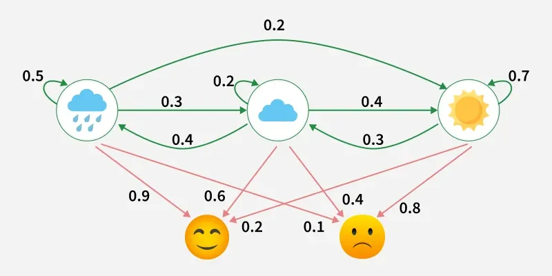
This example shows a Hidden Markov Model where the hidden states are weather conditions (Rainy, Cloudy, Sunny) and the observations are emotions (Happy, Neutral, Sad).
- The green arrows represent transition probabilities, showing how likely the weather is to change from one state to another each day.
- Red arrows represent emission probabilities, showing how likely each emotion is given the current weather.
- Since we only observe the emotions and not the actual weather, the HMM helps infer the most probable hidden weather pattern behind those observations.
Assumptions of HMM
**1. Hidden States
- The actual state of the system is not visible.
- **Example: Weather (Sunny/Rainy) is hidden.
**2. Observations
- We only see the outcomes produced by the hidden states.
- **Example: Friend’s mood (Happy/Sad) is observed.
**3. Markov Property
The model assumes the future state depends only on the current state not on the entire history.
A Hidden Markov Model is defined by
\lambda = (A, B, \pi)
**where
- \boldsymbol{A} (Transition Matrix): Probability of moving from one hidden state to another.
- \boldsymbol{B} (Emission Matrix): Probability of observing a symbol given a hidden state.
- \boldsymbol{\pi} (Initial State Distribution): Probability of starting in each hidden state.
**1. Hidden States (N): These are the internal states of the system, which are not directly observable.
**2. Observations (M): These are the visible outputs generated by the hidden states.
3. Initial State Distribution (\pi): Represents the probability of starting in each hidden state.
**4. Transition Probabilities (A): Defines the probability of moving from one hidden state to another.
**5. Emission Probabilities (B): Defines the probability of producing a particular observed output from a given hidden state.
Hidden Markov Models solve three core problems related to sequences of observations generated by hidden states.
**1. Evaluation Problem (Forward Algorithm)
**Problem: How to compute the probability of an observation sequence?
Mathematically, given an observation sequence:
O = \{o_1, o_2, \dots, o_T\}
and a model:
\lambda = (A, B, \pi)
we compute:
\mathbf{P}(O \mid \lambda) = \sum_{\text{all state sequences } Q} \mathbf{P}(O, Q \mid \lambda)
Because summing over all possible state sequences is computationally expensive, the Forward Algorithm efficiently computes this probability using dynamic programming with the forward variable:
\alpha_t(j) = \mathbf{P}(o_1, o_2, \dots, o_t, q_t = j \mid \lambda)
2. Decoding Problem (Viterbi Algorithm)
**Problem: How to find the most likely hidden state sequence that explains the observations?
Mathematically, it finds:
Q^* = \arg \max_{Q} \mathbf{P}(Q \mid O, \lambda)
The Viterbi Algorithm efficiently computes this using dynamic programming by keeping track of the maximum probability path to each state at each time step.
3. Learning Problem (Baum–Welch Algorithm / EM)
**Problem: How to train the HMM to fit the observed data?
Here, the goal is to estimate the model parameters that maximize the likelihood of the observation sequence:
\lambda_{\text{new}} = \arg \max_{\lambda} \mathbf{P}(O \mid \lambda)
The Baum Welch Algorithm (a type of Expectation-Maximization) iteratively updates estimates of A, B and \pi using the state occupancy probabilities and transition probabilities computed from the observation sequence.
HMM Algorithm
**Step 1 Define State and Observation Space
- **Hidden States: Possible internal states the system can be in.
- **Observations: Visible outputs generated by hidden states.
Step 2 Define Initial State Distribution (\pi): Set probabilities of starting in each hidden state.
**Step 3 Define Transition Matrix (A): Set probabilities for moving from one hidden state to another.
**Step 4 Define Emission Matrix (B): Set probabilities for each observation being emitted by a hidden state.
**Step 5 Train Model: Estimate model parameters using:
- **Baum Welch Algorithm: Trains HMM by estimating A, B,\pi.
- **Forward Backward Algorithm: Computes hidden state probabilities efficiently.
**Step 6 Decode Hidden States: Determine the most likely hidden state sequence using the Viterbi algorithm.
**Step 7 Evaluate Model Performance: Measure model accuracy using metrics like Accuracy, Precision and Recall.
Step-By-Step Implementation
Step 1: Import Libraries
- numpy for arrays and random choices.
- matplotlib and seaborn for plotting.
- hmmlearn for Hidden Markov Models. Python `
import numpy as np import matplotlib.pyplot as plt import seaborn as sns from hmmlearn import hmm
`
Step 2: Define Markov Chain States & Transition Matrix
- Define all possible states in the chain.
- Specify transition probabilities between states.
- Used to simulate a simple Markov process before introducing HMM. Python `
states = ["Sunny", "Rainy"]
transition_matrix = np.array([
[0.8, 0.2],
[0.4, 0.6]
])
print("\nTransition Matrix:") print(transition_matrix)
`
Step 3: Simulate Markov Chain Sequence
- Generate a sequence of states using the transition matrix.
- Start from an initial state.
- Randomly choose next states according to transition probabilities. Python `
def simulate_markov_chain(start_state, n_steps=20): current_state = states.index(start_state) sequence = [start_state] for _ in range(n_steps): current_state = np.random.choice([0, 1], p=transition_matrix[current_state]) sequence.append(states[current_state]) return sequence
mc_sequence = simulate_markov_chain("Sunny", 15) print("\nGenerated Markov Chain Sequence:") print(mc_sequence)
`
Step 4: Define HMM Parameters
- Define hidden states and observations for the HMM.
- Set initial state probabilities, transition matrix and emission matrix.
- These parameters define the behavior of the HMM. Python `
hidden_states = ["Hot", "Cold"] observations = ["IceCream", "Coffee"]
model = hmm.MultinomialHMM(n_components=2, n_iter=50)
model.transmat_ = np.array([
[0.7, 0.3],
[0.4, 0.6]
])
model.emissionprob_ = np.array([
[0.8, 0.2],
[0.3, 0.7]
])
model.startprob_ = np.array([0.6, 0.4])
print("\nTransition Matrix (Hidden States):") print(model.transmat_) print("\nEmission Matrix:") print(model.emissionprob_)
`
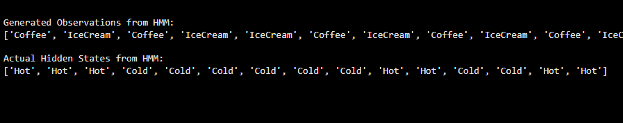
Step 5: Generate Observations from HMM
- Sample sequences of observations and hidden states from the HMM.
- Convert numerical sequences to readable labels.
- Helps to understand how HMM produces observable data. C++ `
model.n_trials = 1 obs_seq, hidden_seq = model.sample(15)
obs_seq = obs_seq.flatten() hidden_seq = hidden_seq.flatten()
decoded_obs = [observations[i] for i in obs_seq] decoded_hidden = [hidden_states[i] for i in hidden_seq]
print("\nGenerated Observations from HMM:") print(decoded_obs) print("\nActual Hidden States from HMM:") print(decoded_hidden)
`
**Output:
Step 6: Decode Hidden States Using Viterbi
- Use the Viterbi algorithm to predict the most likely hidden states.
- Converts observed sequences into inferred hidden states. Python `
n_observations = len(observations) X_decoded = np.zeros((len(obs_seq), n_observations)) X_decoded[np.arange(len(obs_seq)), obs_seq] = 1
logprob, predicted_states = model.decode(X_decoded, algorithm="viterbi") decoded_predicted = [hidden_states[i] for i in predicted_states]
print("\nPredicted Hidden States (Viterbi):") print(decoded_predicted)
`
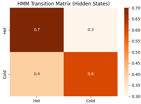
Step 7: Visualize HMM Transition Matrix
- Heatmap helps in understanding transition probabilities between hidden states.
- Useful for analysis and debugging of HMM parameters. Python `
plt.figure(figsize=(6,4)) sns.heatmap(model.transmat_, annot=True, cmap="Oranges", xticklabels=hidden_states, yticklabels=hidden_states) plt.title("HMM Transition Matrix (Hidden States)") plt.show()
`
**Output:
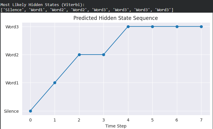
Step 8: Custom Speech-Like HMM Example
- Define multiple hidden states representing speech segments.
- Define observations like “Loud” and “Soft” sounds.
- Predict most likely hidden states using Viterbi and visualize sequence. Python `
states = ["Silence", "Word1", "Word2", "Word3"] n_states = len(states) observations = ["Loud", "Soft"] n_observations = len(observations)
start_probability = np.array([0.8, 0.1, 0.1, 0.0]) transition_probability = np.array([ [0.7, 0.2, 0.1, 0.0], [0.0, 0.6, 0.4, 0.0], [0.0, 0.0, 0.6, 0.4], [0.0, 0.0, 0.0, 1.0] ]) emission_probability = np.array([ [0.7, 0.3], [0.4, 0.6], [0.6, 0.4], [0.3, 0.7] ])
model2 = hmm.CategoricalHMM(n_components=n_states) model2.startprob_ = start_probability model2.transmat_ = transition_probability model2.emissionprob_ = emission_probability
observations_sequence = np.array([0,1,0,0,1,1,0,1]).reshape(-1,1) hidden_states_predicted = model2.predict(observations_sequence)
print("Most Likely Hidden States (Viterbi):") print([states[i] for i in hidden_states_predicted])
sns.set_style("darkgrid") plt.figure(figsize=(8,4)) plt.plot(hidden_states_predicted, "-o") plt.yticks(range(n_states), states) plt.title("Predicted Hidden State Sequence") plt.xlabel("Time Step") plt.show()
`
**Output:
You can download full code from here.
Applications
- **Bioinformatics: Models DNA/protein sequences for gene identification and protein classification.
- **Finance: Capture hidden market states to predict trends and detect bullish/bearish periods.
- **NLP: Perform POS tagging, NER and early machine translation using sequential text modeling.
- **IoT and Cybersecurity: Detect anomalous event sequences in sensors or logs.
- **Weather Forecasting: Predict future weather patterns from historical data sequences.
- **Activity Recognition in Wearables: Classify activities like walking, running or sleeping using sensor
Advantages
- **Easy to Interpret: Clear probabilistic structure of hidden states and observations.
- **Works Well on Small Datasets: Requires less data compared to deep learning models.
- **Fast Inference: Efficient algorithms like Forward and Viterbi enable quick computation.
- **Strong for Anomaly Detection: Can detect unusual sequences effectively.
- **Mathematically Elegant: Solid foundation in probability and statistics.
Limitations
- **Markov Assumption: Only considers the previous state, limiting long-range dependencies.
- **Discrete Hidden States: Struggles with continuous or non-categorical hidden states.
- **Difficulty with Complex Sequences: Less effective than RNNs or LSTMs on complex sequences.
- **Limited Long-Term Memory: Cannot remember distant past events effectively.
- **Less Accurate for High-Dimensional Inputs: Performance drops with high-dimensional data.