Implementation of Lasso Regression From Scratch using Python (original) (raw)

Last Updated : 23 Mar, 2026

Lasso Regression is a regularized linear regression technique used to improve model generalization and handle high-dimensional data efficiently. It balances prediction accuracy and model simplicity by penalising large coefficient values during training.

Adds an L1 penalty term to the loss function, which constrains the magnitude of regression coefficients.
Encourages sparsity in the model by shrinking some coefficients exactly to zero, effectively performing feature selection.
Controls model complexity through the regularization parameter (\lambda), helping reduce overfitting and improve prediction stability.

How Lasso Regression Works

Lasso Regression is an extension of Linear Regression that uses the same hypothesis (prediction) function but modifies the objective function by introducing regularisation. Lasso modifies this objective by adding an L1 regularization term:

J = \sum_{i=1}^{m} \left( y^{i} - h(x^{i}) \right)^2 + \lambda \sum_{j=1}^{n} |w_j|

where:

y^{i}: actual target value for the ith training example
h(x^{i}): predicted value
w_{j}: weight (coefficient) of the jth feature
\lambda: regularization strength

The model minimizes prediction error while penalizing large coefficients, balancing accuracy with simplicity to produce a more generalizable model.

Understanding the Regularization Strength (\lambda)

The regularization strength determines how strongly the model penalizes large coefficients during training.

\lambda = 0: Lasso behaves exactly like Linear Regression
Small \lambda: Slight shrinkage of coefficients
Large \lambda: More coefficients shrink toward zero
Very large \lambda: All coefficients become zero

As \lambda increases, the model applies stronger regularization, which increases bias but reduces variance and makes the model sparser. This balance between bias and variance helps prevent overfitting and improves generalization.

Step By Step Implementation

Here we implement Lasso Regression from scratch in Python using a dataset of employees with Years of Experience and Salary. The model learns the relationship between experience and salary while applying L1 regularization to control overfitting and improve prediction accuracy.

Step 1: Import Required Libraries

Import necessary libraries NumPy, Pandas, train_test_split, StandardScaler and Matplotlib for implementing and visualizing the Lasso Regression model.

Python `

import numpy as np import pandas as pd from sklearn.model_selection import train_test_split from sklearn.preprocessing import StandardScaler import matplotlib.pyplot as plt

Step 2: Define the Lasso Regression Class

Here we create a custom LassoRegression class that implements L1 regularization using gradient descent. This class includes methods for training the model, updating weights and making predictions.

**__init__(): Initializes learning rate, number of iterations and L1 penalty parameter.
**fit(): Trains the model by initializing weights and repeatedly updating them using gradient descent.
**update_weights(): Computes gradients with L1 penalty and updates the weight and bias values.
**predict(): Generates predicted values using the learned weights and bias. Python `

class LassoRegression(): def init(self, learning_rate, iterations, l1_penalty): self.learning_rate = learning_rate self.iterations = iterations self.l1_penalty = l1_penalty

def fit(self, X, Y):
    self.m, self.n = X.shape
    self.W = np.zeros(self.n)
    self.b = 0
    self.X = X
    self.Y = Y

    for i in range(self.iterations):
        self.update_weights()
    return self

def update_weights(self):
    Y_pred = self.predict(self.X)
  
    dW = np.zeros(self.n)
    for j in range(self.n):
        if self.W[j] > 0:
            dW[j] = (-2 * (self.X[:, j]).dot(self.Y - Y_pred) +
                     self.l1_penalty) / self.m
        else:
            dW[j] = (-2 * (self.X[:, j]).dot(self.Y - Y_pred) -
                     self.l1_penalty) / self.m

    db = -2 * np.sum(self.Y - Y_pred) / self.m

    self.W = self.W - self.learning_rate * dW
    self.b = self.b - self.learning_rate * db
    return self

def predict(self, X):
    return X.dot(self.W) + self.b

Step 3: Load the Dataset

Load the dataset using Pandas and display the first few rows.

You can download dataset from here.

Python `

df = pd.read_csv("Experience-Salary.csv") df.head()

**Output:

Screenshot-2026-03-02-145535

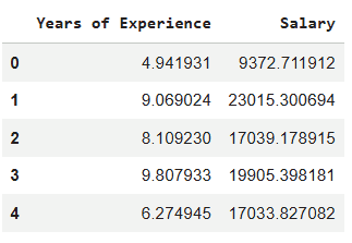
Dataset

Step 4: Prepare and Split the Dataset

Here we separate the feature and target variables, standardize the input data and split the dataset for training and testing.

X contains the input feature (Years of Experience) and Y contains the target variable (Salary).
StandardScaler() is applied to normalize the feature values before training.
train_test_split() divides the data into training and testing sets to evaluate model performance. Python `

X = df.iloc[:, :-1].values Y = df.iloc[:, 1].values scaler = StandardScaler() X = scaler.fit_transform(X) X_train, X_test, Y_train, Y_test = train_test_split( X, Y, test_size=1/3, random_state=0)

Step 5: Train the Lasso Regression Model

Here we initialize the Lasso Regression model with the specified learning rate, number of iterations and L1 penalty. The model is then trained using the training dataset to learn the relationship between experience and salary.

Python `

model = LassoRegression(iterations=1000, learning_rate=0.01, l1_penalty=500) model.fit(X_train, Y_train)

Step 6: Model Evaluation and Output

In this step, we generate predictions using the trained model and examine the learned parameters.

model.predict(X_test) is used to predict salary values and compare them with the actual test values.
The trained weight (W) and bias (b) are printed to observe how the model has learned the relationship between experience and salary. Python `

Y_pred = model.predict(X_test) print("Predicted values: ", np.round(Y_pred[:3], 2)) print("Real values: ", Y_test[:3]) print("Trained W: ", round(model.W[0], 2)) print("Trained b: ", round(model.b, 2))

**Output:

Predicted values: [35539.41 18099.76 43796.5 ]
Real values: [42328.57198221 16443.83637617 44375.48684823]
Trained W: 11516.31
Trained b: 26129.99

Step 7: Visualize the Regression Results

Now we plot the actual salaries against the predicted values to visualize how well the Lasso Regression model fits the data.

Python `

plt.scatter(X_test, Y_test, color='blue', label='Actual Data') plt.plot(X_test, Y_pred, color='yellow', label='Lasso Regression Line') plt.title('Salary vs Experience (Lasso Regression)') plt.xlabel('Years of Experience (Standardized)') plt.ylabel('Salary') plt.legend() plt.show()

**Output:

Screenshot-2026-03-02-150333

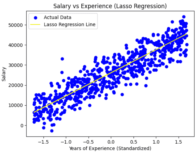
Output

This output shows that the Lasso Regression model fits the data well, capturing the linear relationship between experience and salary. The close match between predicted and actual values demonstrates the model’s effectiveness in learning salary patterns.

Download code from here.