Implementation of Ridge Regression from Scratch using Python (original) (raw)

Last Updated : 9 Jun, 2026

Ridge Regression ( or L2 Regularization ) is a variation of Linear Regression. In Linear Regression, it minimizes the Residual Sum of Squares ( or RSS or cost function ) to fit the training examples perfectly as possible. The cost function is also represented by

J = \frac{1}{m} \sum_{i=1}^{m} \left( y^{(i)} - h(x^{(i)}) \right)^2

Here:

h(x^{(i)}) represents the hypothetical function for prediction.
y^{(i)} actual target value
m total number of training examples

Ridge Regression

Adds an L2 regularization penalty to the cost function
Penalizes large coefficient values to reduce overfitting
Handles multicollinearity more effectively and improves model generalization

**The modified cost function is:

\frac{1}{m}\left[\sum_{i=1}^{m}\left(y^{(i)}-h\left(x^{(i)}\right)\right)^{2}+\lambda \sum_{j=1}^{n} w_{j}^{2}\right]

**Here:

w_j represents the weight for jth feature.
n is the number of features in the dataset.

Working

During gradient descent, Ridge Regression adds an L2 penalty term to the cost function, which reduces the magnitude of the model weights and prevents them from becoming excessively large. By shrinking the weights toward zero, the model becomes simpler, more generalized and less prone to overfitting.

The strength of this regularization is controlled by the hyperparameter λ, which shrinks all weights uniformly.

If λ = 0 : Ridge Regression becomes equivalent to Linear Regression
If λ → ∞: All weights approach zero, leading to an overly simple (underfit) model

Hence, λ should be chosen carefully between these extremes to balance bias and variance.

**Implementation

**1. Import Required Libraries

The required libraries are imported for different tasks such as numerical computations using NumPy, data handling and processing using Pandas, data visualization using Matplotlib and splitting the dataset into training and testing sets using train_test_split.

Python `

import numpy as np import pandas as pd import matplotlib.pyplot as plt from sklearn.model_selection import train_test_split

**2. Creating Class

A custom Ridge Regression model is created using gradient descent. The model includes L2 regularization to reduce overfitting and improve generalization.

Python `

class RidgeRegression:

def __init__(self, learning_rate=0.01, iterations=1000, l2_penalty=1):
    self.learning_rate = learning_rate
    self.iterations = iterations
    self.l2_penalty = l2_penalty

# Train model
def fit(self, X, Y):

    self.m, self.n = X.shape

    # Initialize weights and bias
    self.W = np.zeros(self.n)
    self.b = 0

    # Gradient Descent
    for _ in range(self.iterations):

        Y_pred = self.predict(X)

        # Calculate gradients
        dW = (-2 * X.T.dot(Y - Y_pred) +
              2 * self.l2_penalty * self.W) / self.m

        db = -2 * np.sum(Y - Y_pred) / self.m

        # Update weights
        self.W -= self.learning_rate * dW
        self.b -= self.learning_rate * db

# Predict values
def predict(self, X):
    return X.dot(self.W) + self.b

**3. Load and Prepare the Dataset

The salary dataset is loaded using Pandas. The input feature (X) contains years of experience, while the target variable (Y) contains salary values. The dataset is then split into training and testing sets.

You can download the dataset from here.

Python `

df = pd.read_csv("salary_data.csv")

Features and Target

X = df.iloc[:, :-1].values Y = df.iloc[:, 1].values

Split dataset

X_train, X_test, Y_train, Y_test = train_test_split(X, Y, test_size=0.3, random_state=0)

**4. Model training

An instance of the Ridge Regression model is created and trained using the training dataset.

Python `

Create model

model = RidgeRegression()

Train model

model.fit(X_train, Y_train)

**5. Prediction

The trained model predicts salary values for the test dataset. The predicted values are then compared with the actual salary values.

Python `

Y_pred = model.predict(X_test)

Results

print("Predicted Values :", np.round(Y_pred[:3], 2)) print("Actual Values :", Y_test[:3])

print("Weight :", round(model.W[0], 2)) print("Bias :", round(model.b, 2))

**Output:

Predicted Values : [ 40773.44 123061.09 65085.7 ]

Actual Values : [ 37731. 122391. 57081.]

Weight : 9350.87 Bias : 26747.13

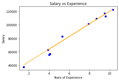
**6. Visualize the Regression Line

A graph is plotted to visualize the actual test data and the regression line generated by the Ridge Regression model.

Python `

plt.scatter(X_test, Y_test, color="blue") plt.plot(X_test, Y_pred, color="red")

plt.title("Salary vs Experience") plt.xlabel("Years of Experience") plt.ylabel("Salary")

plt.show()

Visualization

You can download the source code from here.

Ridge regression leads to dimensionality reduction which makes it a computationally efficient model.