Regularization in Machine Learning (original) (raw)

Last Updated : 30 Apr, 2026

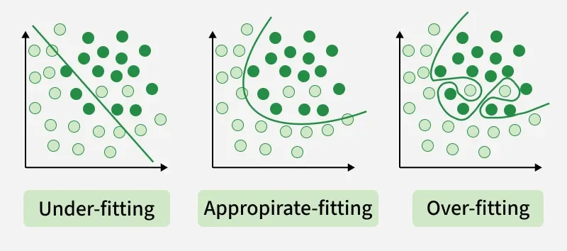
Regularization is a technique used in machine learning to prevent overfitting, which otherwise causes models to perform poorly on unseen data. By adding a penalty for complexity, regularization encourages simpler and more generalizable models.

• **Prevents overfitting: Adds constraints to the model to reduce the risk of memorizing noise in the training data.
• **Improves generalization: Encourages simpler models that perform better on new, unseen data.

Regularization in Machine Learning

Types of Regularization

There are mainly 3 types of regularization techniques, each applying penalties in different ways to control model complexity and improve generalization.

1. Lasso Regression

A regression model which uses the L1 Regularization technique is called LASSO (Least Absolute Shrinkage and Selection Operator) regression. It adds the absolute value of magnitude of the coefficient as a penalty term to the loss function(L). This penalty can shrink some coefficients to zero which helps in selecting only the important features and ignoring the less important ones.

\rm{Cost} = \frac{1}{n}\sum_{i=1}^{n}(y_i-\hat{y_i})^2 +\lambda \sum_{j=1}^{m}{|w_j|}

Where

• m: Number of Features
• n: Number of Examples
• y_i : Actual Target Value
• \hat{y}_i: Predicted Target Value

**Note: These formulas apply to linear models. In neural networks, the number of weights is much larger than the number of features, but the same regularization principles (L1, L2) still apply on all weights.

Lets see how to implement this using python:

• **X, y = make_regression(n_samples=100, n_features=5, noise=0.1, random_state=42): Generates a regression dataset with 100 samples, 5 features and some noise.
• **X_train, X_test, y_train, y_test = train_test_split(X, y, test_size=0.2, random_state=42): Splits the data into 80% training and 20% testing sets.
• **lasso = Lasso(alpha=0.1): Creates a Lasso regression model with regularization strength alpha set to 0.1. Python `

from sklearn.linear_model import Lasso from sklearn.model_selection import train_test_split from sklearn.datasets import make_regression from sklearn.metrics import mean_squared_error

X, y = make_regression(n_samples=100, n_features=5, noise=0.1, random_state=42) X_train, X_test, y_train, y_test = train_test_split(X, y, test_size=0.2, random_state=42)

lasso = Lasso(alpha=0.1) lasso.fit(X_train, y_train)

y_pred = lasso.predict(X_test)

mse = mean_squared_error(y_test, y_pred) print(f"Mean Squared Error: {mse}")

print("Coefficients:", lasso.coef_)

`

**Output:

Lasso Regression

The output shows the model's prediction error and the importance of features with some coefficients reduced to zero due to L1 regularization.

2. Ridge Regression

A regression model that uses the L2 regularization technique is called Ridge regression. It adds the squared magnitude of the coefficient as a penalty term to the loss function(L). It handles multicollinearity by shrinking the coefficients of correlated features, reducing their variance and preventing any single feature from dominating the model.

\rm{Cost} = \frac{1}{n}\sum_{i=1}^{n}(y_i-\hat{y}_i)^2 + \lambda \sum_{j=1}^{m}{w_j^2}

Where,

• n: Number of examples or data points
• m: Number of features i.e predictor variables
• y_i: Actual target value for the ith example
• \hat{y}_i​: Predicted target value for the ith example
• w_i: Coefficients of the features
• \lambda: Regularization parameter that controls the strength of regularization

Lets see how to implement this using python:

• **ridge = Ridge(alpha=1.0): Creates a Ridge regression model with regularization strength alpha set to 1.0. Python `

from sklearn.linear_model import Ridge from sklearn.datasets import make_regression from sklearn.model_selection import train_test_split from sklearn.metrics import mean_squared_error

X, y = make_regression(n_samples=100, n_features=5, noise=0.1, random_state=42) X_train, X_test, y_train, y_test = train_test_split(X, y, test_size=0.2, random_state=42)

ridge = Ridge(alpha=1.0) ridge.fit(X_train, y_train) y_pred = ridge.predict(X_test)

mse = mean_squared_error(y_test, y_pred) print("Mean Squared Error:", mse) print("Coefficients:", ridge.coef_)

`

**Output:

Ridge Regression

The output shows the MSE showing model performance. Lower MSE means better accuracy. The coefficients reflect the regularized feature weights.

3. Elastic Net Regression

Elastic Net Regression is a combination of both L1 as well as L2 regularization. It combines both L1 (absolute values) and L2 (squared values) penalties on the coefficients. With the help of an extra hyperparameter that controls the ratio of the L1 and L2 regularization.

\rm{Cost} = \frac{1}{n}\sum_{i=1}^{n}(y_i-\hat{y}_i)^2 + \lambda \left( (1-\alpha)\sum_{j=1}^{m}|w_j| + \alpha \sum_{j=1}^{m}{w_j^2} \right)

Where

• n: Number of examples (data points)
• m: Number of features (predictor variables)
• y_i:​ Actual target value for the i^{th} example
• \hat{y}_i​: Predicted target value for the ith example
• wi: Coefficients of the features
• \lambda: Regularization parameter that controls the strength of regularization
• \alpha: Mixing parameter where 0 \leq \alpha \leq 1 and \alpha= 1 corresponds to Lasso (L_1) regularization, \alpha= 0 corresponds to Ridge (L_2) regularization and Values between 0 and 1 provide a balance of both L1 and L2 regularization

Lets see how to implement this using python:

• **model = ElasticNet(alpha=1.0, l1_ratio=0.5) : Creates an Elastic Net model with regularization strength alpha=1.0 and L1/L2 mixing ratio 0.5. Python `

from sklearn.linear_model import ElasticNet from sklearn.datasets import make_regression from sklearn.model_selection import train_test_split from sklearn.metrics import mean_squared_error

X, y = make_regression(n_samples=100, n_features=10, noise=0.1, random_state=42) X_train, X_test, y_train, y_test = train_test_split(X, y, test_size=0.2, random_state=42)

model = ElasticNet(alpha=1.0, l1_ratio=0.5) model.fit(X_train, y_train)

y_pred = model.predict(X_test) mse = mean_squared_error(y_test, y_pred)

print("Mean Squared Error:", mse) print("Coefficients:", model.coef_)

`

**Output:

Elastic Net Regression

The output shows MSE which measures how far off predictions are from actual values (lower is better) and coefficients show feature importance.

Benefits of Regularization

Now, let’s see various benefits of regularization which are as follows:

• **Prevents Overfitting: Regularization helps models focus on underlying patterns instead of memorizing noise in the training data.
• **Enhances Performance: Prevents excessive weighting of outliers or irrelevant features helps in improving overall model accuracy.
• **Stabilizes Models: Reduces sensitivity to minor data changes which ensures consistency across different data subsets.
• **Prevents Complexity: Keeps model from becoming too complex which is important for limited or noisy data.
• **Handles Multicollinearity: Reduces the magnitudes of correlated coefficients helps in improving model stability.
• **Promotes Consistency: Ensures reliable performance across different datasets which reduces the risk of large performance shifts.

Learn more about the difference between the regularization techniques here: **Lasso vs Ridge vs Elastic Net