Factor Analysis (original) (raw)

Last Updated : 8 Apr, 2026

Factor Analysis is a statistical technique used in data analysis to identify hidden patterns or underlying relationships among a large set of variables. It helps reduce data complexity by grouping correlated variables into smaller sets called factors which represent shared characteristics or dimensions within the data.

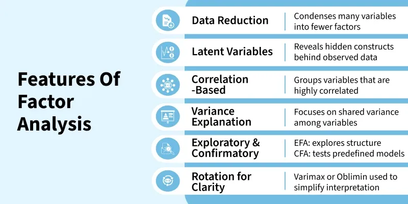
Features

Factor analysis serves several purposes and objectives in statistical analysis:

1. **Dimensionality Reduction: Simplifies datasets by grouping correlated variables into fewer factors making data easier to interpret.
2. **Identifying Latent Constructs: Reveals hidden variables like traits, attitudes that explain observed patterns.
3. **Data Summarization: Summarizes many variables into a concise set of factors while retaining key information.
4. **Hypothesis Testing: Evaluates whether the data support expected relationships among variables.
5. **Variable Selection: Highlights the most relevant variables for analysis or modelling.
6. **Improving Models: Reduces multicollinearity and enhances predictive model performance.

Commonly Used Terms in Factor Analysis

Most commonly used terms in factor analysis are:

1. **Factors: Hidden variable that explains patterns among observed variables.
2. **Factor Loading: Strength of the relationship between a variable and a factor.
3. **Eigenvalue: Amount of variance explained by each factor.
4. **Communalities: Explains how much of a variable’s variance is explained by the extracted factors.
5. **Rotation: Technique to make factors more interpretable like Varimax.
6. **Scree Plot: A plot used to determine the number of factors to retain based on the magnitude of eigenvalues.
7. **Kaiser-Meyer-Olkin (KMO) Measure: It checks if your data is suitable for factor analysis, values closer to 1 mean the data is a good fit.

Types of Factor Analysis

There are two main types of Factor Analysis used during Data Analysis:

1. Exploratory Factor Analysis (EFA)

• Identifies underlying structure without prior assumptions.
• Groups correlated variables into factors organically.
• Helps determine the number of factors needed.
• Used when relationships among variables are unknown.

2. Confirmatory Factor Analysis (CFA)

• Tests specific, theory driven hypotheses about variable factor relationships.
• Uses structural equation modeling to check model fit.
• Accounts for measurement error.
• Used when factor structure is already hypothesized.

Some of the types of Factor Extraction methods are:

1. Principal Component Analysis (PCA)

• Principal Component Analysis aims to extract factors that account for the maximum possible variance in the observed variables.
• Factor weights are computed to extract successive factors until no further meaningful variance can be extracted.
• After extraction, the factor model is often rotated for further analysis to enhance interpretability.

2. Canonical Factor Analysis

• Also known as Rao's canonical factoring, this method computes a similar model to PCA but uses the principal axis method.
• Seeks factors that have the highest canonical correlation with the observed variables.
• Canonical factor analysis is not affected by arbitrary rescaling of the data making it robust to certain data transformations.

3. Common Factor Analysis

• It's also referred to as Principal Factor Analysis (PFA) or Principal Axis Factoring (PAF).
• This method aims to identify the fewest factors necessary to account for the variance among a set of variables.
• Unlike PCA, common factor analysis focuses on capturing shared variance rather than overall variance.

Assumptions of Factor Analysis

Some of the assumptions of factorial analysis are as follows:

1. **Linearity: The relationships between variables and factors are assumed to be linear.
2. **Multivariate Normality: The variables in the dataset should follow a multivariate normal distribution.
3. **No Multicollinearity: Variables should not be highly correlated with each other as high multicollinearity can affect the stability and reliability of the factor analysis results.
4. **Homoscedasticity: The variance of the variables should be roughly equal across different levels of the factors.
5. **Independent Observations: The observations in the dataset should be independent of each other.
6. **Linearity of Factor Scores: The relationship between the observed variables and the latent factors is assumed to be linear even though the observed variables may not be linearly related to each other.

Working of Factor Analysis

Here are the general steps involved in conducting a factor analysis:

1. **Determine the Suitability of Data for Factor Analysis

• **Bartlett's Test: Check the significance level to determine if the correlation matrix is suitable for factor analysis.
• **Kaiser Meyer Olkin (KMO) Measure: Verify the sampling adequacy. A value greater than 0.6 is generally considered acceptable.
• **Principal Component Analysis (PCA): Used when the main goal is data reduction.
• **Principal Axis Factoring (PAF): Used when the main goal is to identify underlying factors.
• Use the chosen extraction method to identify the initial factors.
• Extract eigenvalues to determine the number of factors to retain. Factors with eigenvalues greater than 1 are typically retained in the analysis.
• Compute the initial factor loadings.

4. **Determine the Number of Factors to Retain

• **Scree Plot: Plot the eigenvalues in descending order to visualize the point where the plot levels off the "elbow" to determine the number of factors to retain.
• **Eigenvalues: Retain factors with eigenvalues greater than 1.

5. **Factor Rotation

• **Orthogonal Rotation (Varimax, Quartimax): Assumes that the factors are uncorrelated.
• **Oblique Rotation (Promax, Oblimin): Allows the factors to be correlated.
• Rotate the factors to achieve a simpler and more interpretable factor structure.
• Examine the rotated factor loadings.

6. **Interpret and Label the Factors

• Analyze the rotated factor loadings to interpret the underlying meaning of each factor.
• Assign meaningful labels to each factor based on the variables with high loadings on that factor.

7. **Compute Factor Scores (if needed)

• Calculate the factor scores for each individual to represent their value on each factor.

8. **Report and Validate the Results

• Report the final factor structure including factor loadings and communalities.
• Validate the results using additional data or by conducting a confirmatory factor analysis if necessary.

Implementation of Factor Analysis

Here's step by step implementation of factor analysis in Python using the factor_analyzer library:

Step 1: Install Dependencies

Installing the factor_analyzer Python library.

Python `

!pip install factor_analyzer

`

Step 2: Import Libraries

Importing libraries like Numpy, Pandas, Matplotlib and factor_analyzer.

Python `

import pandas as pd import numpy as np from factor_analyzer import FactorAnalyzer, calculate_bartlett_sphericity, calculate_kmo import matplotlib.pyplot as plt

`

Step 3: Creating Data

Here we will create random data points for analysis.

• **np.random.rand(50, 6): Creating a 50×6 matrix of random numbers between 0 and 1.
• **pd.DataFrame: Converting it into a DataFrame with column names var1 to var6.
• **np.random.seed(0): Ensuring same random numbers every run. Python `

np.random.seed(0) data = np.random.rand(50, 6) df = pd.DataFrame(data, columns=[f'var{i+1}' for i in range(6)])

`

Step 4: Bartlett's Test of Sphericity

• Testing whether the variables are sufficiently correlated for factor analysis.
• **Chi-square value: Testing statistic.
• **P-value: If < 0.05, factor analysis is appropriate.Since the p-value (0.404) is greater than 0.05, the data is not suitable for factor analysis. Python `

chi_sq, p = calculate_bartlett_sphericity(df) print(f'Chi-square: {chi_sq}, P-value: {p}')

`

**Output:

Chi-square: 15.672036566609192, P-value: 0.40417670251236276

Step 5: KMO Test

1. Measuring sampling adequacy.

2. KMO value ranges:

• **0.8: great
• **0.7–0.8: good
• **0.6–0.7: mediocre
• ****<0.6:** factor analysis may not be suitable Python `

kmo_all, kmo_model = calculate_kmo(df) print(f'KMO: {kmo_model}')

`

**Output:

KMO: 0.5054897167472236

Step 6: Factor Analysis (Eigen Values)

• **FactorAnalyzer(rotation="varimax"): Initializing the factor analysis model with varimax rotation.
• **fit(df): Fitting the model to the data.
• **get_eigenvalues(): Returning eigenvalues of each factor.
• Eigenvalues show how much variance each factor explains. Python `

fa = FactorAnalyzer(rotation="varimax") fa.fit(df) eigen_values, _ = fa.get_eigenvalues()

`

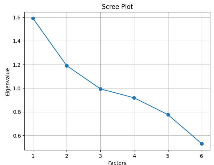
Step 7: Scree Plot

1. Plotting eigenvalues against factor numbers.

2. Scree plot helps determine the optimal number of factors:

• Look for the elbow point where the curve levels off.
• Factors above this point are typically retained. Python `

plt.plot(range(1, df.shape[1]+1), eigen_values, marker='o') plt.title('Scree Plot'); plt.xlabel('Factors'); plt.ylabel('Eigenvalue'); plt.grid(True); plt.show()

`

Step 8: Factor Analysis

• Re-running factor analysis using 2 factors.
• Producing factor loadings, variance explained and scores.
• **Factor Loadings: Showing how strongly each variable loads onto each factor.
• **Factor Variance: Returning variance of each factors and proportion of total variance.
• **Factor Scores: Calculating a score for each observation on each factor. Python `

fa = FactorAnalyzer(n_factors=2, rotation="varimax") fa.fit(df)

print("Factor Loadings:\n", fa.loadings_) print("Factor Variance:\n", fa.get_factor_variance()) print("Factor Scores:\n", fa.transform(df))

`

**Output:

Scree Plot

Applications

1. **Market Research: Identifies patterns in consumer preferences and segments customers for targeted strategies.
2. **Psychology: Reveals latent traits like personality dimensions, attitudes or mental health factors.
3. **Education: Groups exam or survey questions into skill areas or learning domains for better evaluation.
4. **Finance: Detects hidden economic drivers or risk factors influencing markets and investments.
5. **Healthcare: Clusters symptoms or risk indicators into categories to support diagnosis and treatment.

Advantages

• Helps identify hidden patterns and relationships among variables
• Makes complex data easier to interpret and visualize
• Reduces multicollinearity in datasets used for modeling
• Useful for building and validating theoretical constructs
• Reduces a large number of variables into fewer meaningful factors, simplifying analysis

Limitations

• Results depend on choices like number of factors and rotation method
• Requires a sufficiently large dataset for reliable results
• Assumes linear relationships, which may not always hold
• Sensitive to noise and outliers in the data
• Interpretation of factors can sometimes be difficult or ambiguous.