knearest neighbor algorithm using Sklearn Python (original) (raw)

Last Updated : 23 Mar, 2026

K-Nearest Neighbors (KNN) works by identifying the 'k' nearest data points called as neighbors to a given input and predicting its class or value based on the majority class or the average of its neighbors. In this article we will implement it using Python's Scikit-Learn library.

1. **Generating and Visualizing the 2D Data

• We will import libraries like pandas, matplotlib, seaborn and scikit learn.
• The make_moons() function generates a 2D dataset that forms two interleaving half circles.
• This kind of data is non-linearly separable and perfect for showing how k-NN handles such cases. Python `

from sklearn.datasets import make_moons import matplotlib.pyplot as plt import seaborn as sns import pandas as pd

Create synthetic 2D data

X, y = make_moons(n_samples=300, noise=0.3, random_state=42)

Create a DataFrame for plotting

df = pd.DataFrame(X, columns=["Feature 1", "Feature 2"]) df['Target'] = y

Visualize the 2D data

plt.figure(figsize=(8, 6)) sns.scatterplot(data=df, x="Feature 1", y="Feature 2", hue="Target", palette="Set1") plt.title("2D Classification Data (make_moons)") plt.grid(True) plt.show()

`

**Output:

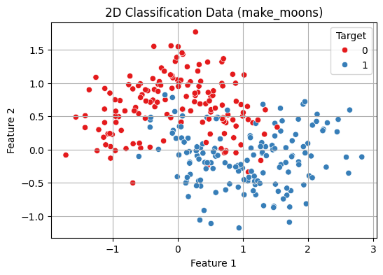
2D Classification Data Visualisation

2. **Train-Test Split and Normalization

• **train_test_split() splits the data into 70% training and 30% testing.
• **random_state=42 ensures reproducibility.
• **stratify=y maintains the same class distribution in both training and test sets which is important for balanced evaluation.
• **StandardScaler() standardizes the features by removing the mean and scaling to unit variance (z-score normalization).
• This is important for distance-based algorithms like k-NN as it ensures all features contribute equally to distance calculations. Python `

from sklearn.model_selection import train_test_split from sklearn.preprocessing import StandardScaler

Split into train and test

X_train, X_test, y_train, y_test = train_test_split( X_scaled, y, test_size=0.3, random_state=42, stratify=y )

Normalize the features

scaler = StandardScaler() X_scaled = scaler.fit_transform(X)

`

3. **Fit the k-NN Model and Evaluate

• This creates a k-Nearest Neighbors (k-NN) classifier with k = 5 meaning it considers the 5 nearest neighbors for making predictions.
• **fit(X_train, y_train) trains the model on the training data.
• **predict(X_test) generates predictions for the test data.
• **accuracy_score() compares the predicted labels (y_pred) with the true labels (y_test) and calculates the accuracy i.e the proportion of correct predictions. Python `

from sklearn.neighbors import KNeighborsClassifier from sklearn.metrics import accuracy_score

Train a k-NN classifier

knn = KNeighborsClassifier(n_neighbors=5) knn.fit(X_train, y_train)

Predict and evaluate

y_pred = knn.predict(X_test) print(f"Test Accuracy (k=5): {accuracy_score(y_test, y_pred):.2f}")

`

**Output:

Test Accuracy (k=5): 0.87

4. **Cross-Validation to Choose Best k

Choosing the optimal k-value is critical before building the model for balancing the model's performance.

• A **smaller k value makes the model sensitive to noise, leading to overfitting (complex models).
• A **larger k value results in smoother boundaries, reducing model complexity but possibly underfitting.

This code performs model selection for the k value in the k-NN algorithm using 5-fold cross-validation:

• It tests values of k from 1 to 20.
• For each k, a new k-NN model is trained and validated using **cross_val_score which automatically splits the dataset into 5 folds, trains on 4 and evaluates on 1, cycling through all folds.
• The mean accuracy of each fold is stored in **cv_scores.
• A line plot shows how accuracy varies with k helping visualize the optimal choice.
• The best_k is the value of k that gives the highest mean cross-validated accuracy. Python `

from sklearn.model_selection import cross_val_score import numpy as np

Range of k values to try

k_range = range(1, 21) cv_scores = []

Evaluate each k using 5-fold cross-validation

for k in k_range: knn = KNeighborsClassifier(n_neighbors=k) scores = cross_val_score(knn, X_scaled, y, cv=5, scoring='accuracy') cv_scores.append(scores.mean())

Plot accuracy vs. k

plt.figure(figsize=(8, 5)) plt.plot(k_range, cv_scores, marker='o') plt.title("k-NN Cross-Validation Accuracy vs k") plt.xlabel("Number of Neighbors: k") plt.ylabel("Cross-Validated Accuracy") plt.grid(True) plt.show()

Best k

best_k = k_range[np.argmax(cv_scores)] print(f"Best k from cross-validation: {best_k}")

`

**Output:

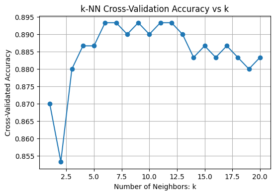
Choosing Best k

Best k from cross-validation: 6

5. **Training with Best k

• The model is trained on the training set with the optimized k (Here k = 6).
• The trained model then predicts labels for the unseen test set to evaluate its real-world performance. Python `

Train final model with best k

best_knn = KNeighborsClassifier(n_neighbors=best_k) best_knn.fit(X_train, y_train)

Predict on test data

y_pred = best_knn.predict(X_test)

`

**6. Evaluate Using More Metrics

• Calculate the confusion matrix comparing true labels (y_test) with predictions (y_pred).
• Use **ConfusionMatrixDisplay to visualize the confusion matrix with labeled classes

Print a classification report that includes:

• **Precision: How many predicted positives are actually positive.
• **Recall: How many actual positives were correctly predicted.
• **F1-score: Harmonic mean of precision and recall.
• **Support: Number of true instances per class. Python `

from sklearn.metrics import confusion_matrix, classification_report, ConfusionMatrixDisplay

Confusion Matrix

cm = confusion_matrix(y_test, y_pred) disp = ConfusionMatrixDisplay(confusion_matrix=cm, display_labels=["Class 0", "Class 1"]) disp.plot(cmap="Blues") plt.title(f"Confusion Matrix (k={best_k})") plt.grid(False) plt.show()

Detailed classification report

print("Classification Report:") print(classification_report(y_test, y_pred, target_names=["Class 0", "Class 1"]))

`

**Output:

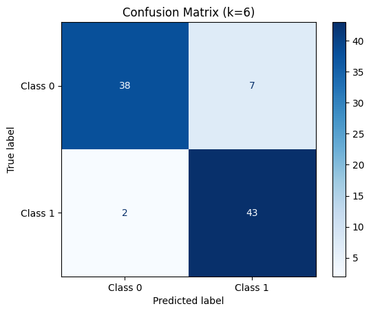
Confusion Matrix for k = 6

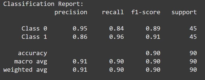
Classification Report

7. **Visualize Decision Boundary with Best k

• Create a 2D mesh grid (xx, yy) covering the feature space.
• Use the trained model (best_knn) to predict class labels for each grid point.
• Reshape predictions to match the grid and plot decision regions using contourf.
• Overlay the original data points using sns.scatterplot to compare true classes with model predictions.

This helps visualize how the model separates classes for the chosen value of k.

Python `

Create mesh grid

x_min, x_max = X_scaled[:, 0].min() - 1, X_scaled[:, 0].max() + 1 y_min, y_max = X_scaled[:, 1].min() - 1, X_scaled[:, 1].max() + 1

xx, yy = np.meshgrid( np.linspace(x_min, x_max, 300), np.linspace(y_min, y_max, 300) )

Predict on mesh grid with best k

Z = best_knn.predict(np.c_[xx.ravel(), yy.ravel()]) Z = Z.reshape(xx.shape)

Plot decision boundary

plt.figure(figsize=(8, 6)) plt.contourf(xx, yy, Z, cmap=plt.cm.coolwarm, alpha=0.3) sns.scatterplot(x=X_scaled[:, 0], y=X_scaled[:, 1], hue=y, palette="Set1", edgecolor='k') plt.title(f"Decision Boundary with Best k = {best_k}") plt.xlabel("Feature 1 (scaled)") plt.ylabel("Feature 2 (scaled)") plt.grid(True) plt.show()

`

**Output:

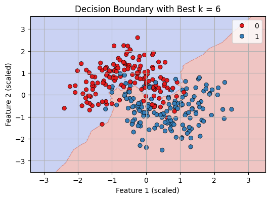
Decision Boundary with best K = 6

We can see that our KNN model is working fine in classifying datapoints.

You can download the complete code from here.