Learning Rate Decay (original) (raw)

Last Updated : 23 Jul, 2025

When training a machine learning model, the learning rate plays a important role in determining how quickly the model adjusts its weights based on the errors it makes. If we start with a learning rate that's too high, the model might learn quickly but could overshoot the best solution. If it's too low, learning can become too slow and the model might get stuck before reaching an optimal solution.

To address this learning rate decay was introduced which helps us adjust the learning rate during training. We start with a higher rate which allows the model to make larger updates and learn faster. As training progresses and the model gets closer to an optimal solution, the learning rate decreases allowing for finer adjustments and better convergence.

Why Use Learning Rate Decay?

• **Faster Training: By starting with a larger learning rate, the model can make quicker progress early in training. This allows the model to learn the general patterns faster, especially when large weight updates are needed in the initial stages.
• **Better Convergence: As the model approaches the optimal solution, smaller learning rates allow for more precise weight updates. This gradual reduction in the learning rate helps the model fine-tune its parameters, preventing overshooting and ensuring it reaches the best possible solution.
• **Improved Generalization: In later stages, the decay helps reduce the risk of overfitting by slowing down the learning process. This more controlled approach helps the model generalize better, ensuring that it performs well not just on the training data but also on unseen data.

Working of Learning Rate Decay

Learning rate decay works similarly to driving toward a parking spot. Initially, we drive fast to cover more distance quickly but as we get closer to our destination, we slow down to park more accurately. In machine learning, this concept translates to starting with a larger learning rate to make faster progress in the beginning and then gradually reducing it to fine-tune the model’s weights in the later stages of training.

The decay is designed to allow the model to make large, broad adjustments early in training and more delicate adjustments as it approaches the optimal solution. This controlled approach helps the model converge more efficiently without overshooting or getting stuck.

There are several methods to implement learning rate decay each with a different approach to how the learning rate decreases over time. Some methods decrease the learning rate in discrete steps while others reduce it more smoothly. The choice of decay method can depend on the task, model and how quickly the learning rate needs to be reduced during training.

Common Types of Learning Rate Decay

There are various methods to reduce the learning rate each has a different approach to the process:

**1. Step Decay: In step decay, the learning rate is reduced by a fixed factor after a predetermined number of epochs. This method is simple but effective.

**Formula: lr = lr_{initial} * drop \;rate^{\frac{epoch}{step\;size}}

**2. Exponential Decay: It reduces the learning rate exponentially at each epoch, leading to a smooth decrease.

**Formula: lr = lr_{initial}\; * \; e^{-decay\;rate \;* \;epoch}

**3. Inverse Time Decay: A factor inversely proportional to the number of epochs is used to reduce the learning rate through inverse decay.

**Formula: lr = lr_{initial} \; * \; \frac{1}{1 + decay * epoch}

**4. Polynomial Decay: It decreases the learning rate based on a polynomial function of the epoch number. This offers a more controlled reduction over time.

**Formula: lr = lr_{initial} \; * \; \left ( 1 - \frac{epoch}{max\;epoch}\right )^{power}

Mathematical Representation of Learning Rate Decay

Understanding the mathematical foundation behind learning rate decay helps clarify how the learning rate is adjusted over time. A basic learning rate decay plan can be mathematically represented as follows:

Assume that the starting learning rate is \eta_{0} and that the learning rate at epoch t is \eta_{t}.

A typical decay schedule for learning rates is based on a constant decay rate \alpha where \alpha \epsilon (0,1), applied at regular intervals (e.g every n epochs). The formula for this basic decay is:

\eta_{t} = \frac{\eta_{0}}{1 + \alpha \cdot t}

Where:

• \eta_{t} is the learning rate at epoch t.
• \eta_{0} is the initial learning rate at the start of training.
• \alpha is the fixed decay rate, typically a small positive value such as 0.1 or 0.01.
• t is the current epoch during training.

In this equation:

• The learning rate \eta_{t} decreases as t increases, means that as the number of epochs grows, the learning rate becomes smaller.
• The decay factor α controls how quickly the learning rate decreases.
• The learning rate is reduced by a percentage of its previous value at each epoch which helps the optimization process.

This schedule provides the optimization by helping the model to converge more quickly at first with larger learning steps and then fine-tuning in smaller increments as it approaches the local minimum.

Implementing Learning Rate Decay

Here we will see how to implement learning rate decay in TensorFlow while building a neural network for classification on the MNIST dataset (a dataset of handwritten digits).

**1. Importing Libraries

We will be using TensorFlow for building and training the model, Keras which is a high-level API within TensorFlow for defining, training and evaluating models and Numpy libraries for this implementation.

Python `

import tensorflow as tf from tensorflow.keras.datasets import mnist from tensorflow.keras.models import Sequential from tensorflow.keras.layers import Dense, Flatten from tensorflow.keras.optimizers import SGD from tensorflow.keras.callbacks import LearningRateScheduler import numpy as np

`

**2. Loading the MNIST Data

The MNIST dataset contains images of handwritten digits and we load it using **TensorFlow’s mnist.load_data() function. The dataset is then split into training and testing sets. Each pixel value is divided by 255.0 to normalize it into a range of 0 to 1.

Python `

(x_train, y_train), (x_test, y_test) = mnist.load_data() x_train, x_test = x_train / 255.0, x_test / 255.0

`

**3. Building the Model

We create a Sequential model using Keras. The model consists of:

• **Flatten Layer: This layer flattens the 28x28 pixel images (which are in a 2D grid) into a 1D array of size 784.
• **Dense Layer (Hidden Layer): This is a fully connected layer with 128 units (neurons) and Rectified Linear Unit activation (ReLU).
• **Dense Layer (Output Layer): The final layer is a Dense layer with 10 units each corresponding to one of the 10 possible classes (digits 0-9). The activation function used here is softmax which converts the raw scores from the network into probabilities. Python `

model = Sequential([ Flatten(input_shape=(28, 28)), Dense(128, activation='relu'), Dense(10, activation='softmax')])

`

**4. Setting up Learning Rate Decay

We define a learning rate schedule that decreases the learning rate over time. Here, we use Exponential Decay where:

• **initial_learning_rate = 0.1 is the starting learning rate.
• **decay_steps = 1000 shows how frequently to apply decay (after 1000 batches).
• **decay_rate = 0.96 is the rate at which the learning rate decays (reduces by 4% after each decay step).
• **staircase=True makes the decay occur in discrete steps rather than continuously. Python `

initial_lr = 0.1 lr_schedule = tf.keras.optimizers.schedules.ExponentialDecay( initial_learning_rate=initial_lr, decay_steps=1000,
decay_rate=0.96,
staircase=True)

`

**5. Compiling the Model

Now we compile the model with:

• **Optimizer: We use SGD (Stochastic Gradient Descent) with the learning rate defined by the **lr_schedule.
• **Loss function: Sparse categorical cross-entropy because we have 10 classes (digits 0-9).
• **Metrics: Accuracy is used as a performance measure during training. Python `

model.compile(optimizer=tf.keras.optimizers.SGD(learning_rate=lr_schedule), loss='sparse_categorical_crossentropy', metrics=['accuracy'])

`

**6. Callback to Print Learning Rate

We define a custom callback to print the learning rate at the start of each epoch. This will help us track how the learning rate changes during training due to the decay schedule.

Python `

class PrintLR(tf.keras.callbacks.Callback): def on_epoch_begin(self, epoch, logs=None): opt = self.model.optimizer if callable(opt.learning_rate): lr = opt.learning_rate(opt.iterations) else: lr = opt.learning_rate print(f"Epoch {epoch+1:02d}: learning rate = {tf.keras.backend.get_value(lr):.5f}")

`

7. Training the Model

The model is trained for 15 epochs. The training process uses the **x_train and **y_train datasets and we validate the model on the **x_test and **y_test datasets.

Python `

model.fit(x_train, y_train, epochs=15, validation_data=(x_test, y_test), callbacks=[PrintLR()], verbose=2)

`

**Output:

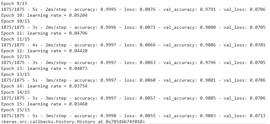
Training the model

8. Evaluating the Model

After training, we evaluate the model’s performance on the test set. The test loss and accuracy are displayed to assess how well the model generalizes to unseen data.

Python `

test_loss, test_accuracy = model.evaluate(x_test, y_test, verbose=2) print('\nTest accuracy:', test_accuracy)

`

**Output:

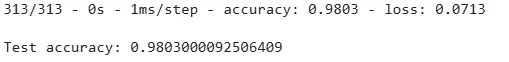
Test accuracy

9. Result

Python `

current_lr = lr_schedule(model.optimizer.iterations) print(f"Current learning rate: {current_lr.numpy()}")

`

**Output:

Current learning rate: 0.031885575503110886

The learning rate will remain constant during the early epochs and gradually decrease according to the exponential decay schedule.

Advantages of Learning Rate Decay

Deep learning and machine learning models are frequently trained using the learning rate decay technique. It provides a number of benefits that support more effective and efficient training including:

• **Improved Convergence: As training goes on, the learning rate is lowered which helps in the models convergence to a better solution. By doing this, it may be avoided that the loss function's minimum is exceeded.
• **Enhanced Generalization: In order to reduce overfitting, a model's capacity to generalize to new data might be enhanced via slower learning rates in later training rounds.
• **Stability: By avoiding significant weight changes that could lead to the model oscillating or diverging, learning rate decay stabilizes training.

Disadvantages of Learning Rate Decay

Despite many benefits to learning rate decay, it's important to be see of any potential drawbacks and difficulties while using it. Considerations and disadvantages are as follows:

• **Complexity: The training process can get more complicated by implementing and choosing the appropriate learning rate decay schedule in big and complex neural networks.
• **Hyperparameter Sensitivity: Hyperparameter tuning is involved in the decay schedule and learning rate selection. Hyperparameter settings or an improper schedule can work against training instead of in favor of it.
• **Delayed Convergence: Aggressive learning rate decay can sometimes make the model converge very slowly which could require more training time.

By mastering learning rate decay, we can significantly improve our model's training efficiency, stability and generalization, ultimately leading to better performance and more reliable results.