ML | Active Learning (original) (raw)

Last Updated : 6 Aug, 2025

Active Learning is a special case of Supervised Machine Learning. This approach is used to construct a high-performance classifier while keeping the size of the training dataset to a minimum by actively selecting the valuable data points.

**Active Learning in Machine Learning

A subset of machine learning known as "active learning" allows a learning algorithm to interactively query a user to label data with the desired outputs. The algorithm actively chooses from the pool of unlabeled data the subset of examples to be labelled next in active learning. The basic idea behind the active learner algorithm concept is that if an ML algorithm could select the data it wants to learn from, it might be able to achieve a higher degree of accuracy with fewer training labels.

How does active learning work?

To enhance a machine learning model, active learning selects the most informative data points iteratively from an unlabeled dataset and requests labels for these points. The main idea is to deliberately select the situations where the model is unsure of itself or where it could most benefit from more information. In contrast to conventional supervised learning, this method aims to lower the labelling cost and enhance the model's performance with fewer labelled examples.

Here's a detailed explanation of how active learning usually works:

Initialization:

• To train an initial machine learning model, start with a small labelled dataset.

Model Training:

• Using the available labelled data, train the first model.

Uncertainty Estimation:

• To predict the unlabeled data, apply the trained model.
• Calculate the model's prediction confidence or uncertainty. Margin, variance, and entropy are examples of common metrics.

Query Technique:

• Choose the cases from the unlabeled pool where the model is unsure or has low confidence.
• Depending on the particular active learning algorithm, the query strategy selected may include picking the cases with the highest level of uncertainty, cases close to the decision boundary, or cases where models in an ensemble disagree.

Labelling:

• Ask an oracle-a human annotator or another source of ground truth labels—for labels for the chosen instances.

Model Update:

• Add the recently annotated data to the training set.
• Using the revised labeled dataset, retrain the model.

Repeat:

• Repeat steps 2 through 6 iteratively until a budget is depleted or a performance threshold is reached.

Key concepts of Active Learning

• **Query Strategy: It is important to have a strategy in place for deciding which instances to query for labels. Diverse approaches concentrate on different elements, like diversity, uncertainty, or representative sampling.
• **Model Uncertainty: Active learning makes use of the uncertainty estimates that models frequently provide to pinpoint situations in which the model is unsure of its predictions.
• **Oracle: The organisation in charge of the ground truth labelling. In actuality, this might be an outside system or a human annotator.
• **Stopping Conditions: A model's performance may plateau, a target accuracy may be met, or the iteration of active learning may end when a predetermined number of labelled examples is reached.

**Where should we apply active learning?

1. We have a very small amount or a huge amount of dataset.
2. Annotation of the unlabeled dataset costs human effort, time, and money.
3. We have access to limited processing power.

**Example

On a certain planet, there are various fruits of different sizes (1-5), some of them are poisonous and others don't. The only criterion to decide whether a fruit is poisonous or not is its size. our task is to train a classifier that predicts whether the given fruit is poisonous or not. The only information we have is a fruit with size 1 is not poisonous, a fruit of size 5 is poisonous and after a particular size, all fruits are poisonous.

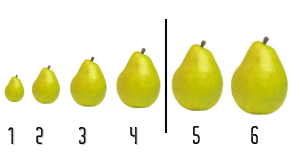
1. The first approach is to check each and every size of the fruit, which consumes time and resources.
2. The second approach is to apply the binary search and find the transition point (decision boundary). This approach uses fewer data and gives the same results as of linear search.

**Active Learning algorithm approaches

**1. Query Synthesis

• Generally, this approach is used when we have a very small dataset.
• This approach we choose any uncertain point from given n-dimensional space. we don't care about the existence of that point.

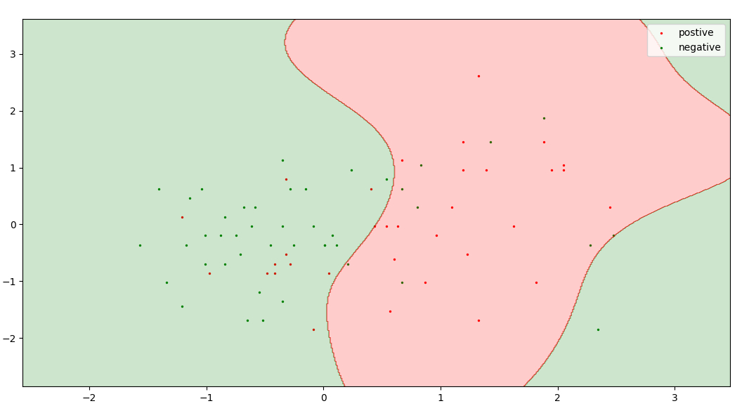
In this query, synthesis can pick any point(valuable) from 3*3 2-D plane.

• Sometimes it would be difficult for human oracle to annotate the queried data point.

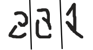
These are some queries generated by the Query Synthesis approach for a model trained for handwritten recognition. It is very difficult to annotate these queries.

**2. Sampling

• This approach is used when we have a large dataset.
• In this approach, we split our dataset into three parts: Training Set; Test Set; Unlabeled Pool(ironical) [5%; 25%, 70%].
• This training dataset is our initial dataset and is used to initially train our model.
• This approach selects valuable/uncertain points from this unlabeled pool, this ensures that all the query can be recognized by human oracle

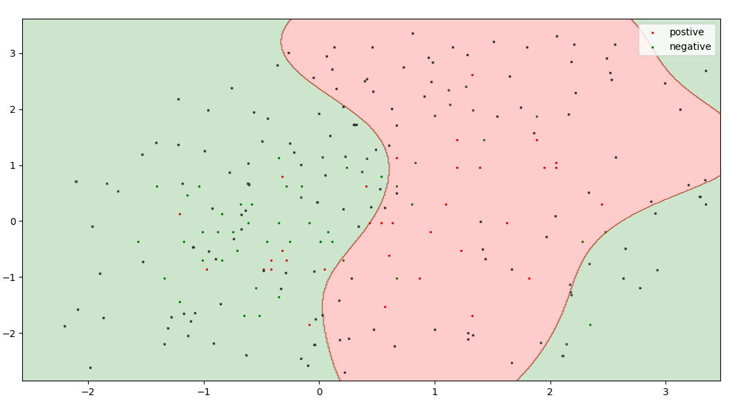
Black points represents unlabeled pool and union red, green colour dots represents training dataset.

Here is an active learning model which decides valuable points on the basis of, the probability of a point present in a class. In Logistic Regression points closest to the threshold (i.e. probability = 0.5) is the most uncertain point. So, I choose the probability between 0.47 to 0.53 as a range of uncertainty.

Benefits of Active Learning

• **Reduced Labeling Costs: By reducing the quantity of labeled data needed for training, active learning helps to cut down on labeling expenses.
• **Enhanced Model Performance: Active learning frequently produces models with higher accuracy and generalization by concentrating on the most instructive examples.
• **Optimal Resource Utilisation: When labeled data acquisition presents a bottleneck, active learning enables a more economical use of resources.
• **Adaptability to Data Distribution: Because active learning allows the model to concentrate on difficult examples, it works well in situations where the distribution of data is uneven or unbalanced.

Code Implementation

1. Importing necessary libraries:

The code imports several Python libraries commonly used in data preprocessing and machine learning tasks. The provided code imports these modules and libraries, preparing the environment for different scikit-learn machine learning tasks and data preprocessing tasks.

Python3 `

import numpy as np import pandas as pd from statistics import mean from sklearn.impute import SimpleImputer from sklearn.preprocessing import StandardScaler from sklearn.linear_model import LogisticRegression from sklearn.model_selection import train_test_split

`

2. Splitting dataset into train and test set:

Dividing the data into training and testing sets. This (train_test_split) function allows you to split your dataset into labeled and unlabeled portions, simulating an active learning setup and allowing you to iteratively query labels for the most informative instances.

Python3 `

split dataset into test set, train set and unlabel pool

def split(dataset, train_size, test_size): x = dataset[:, :-1] y = dataset[:, -1] x_train, x_pool, y_train, y_pool = train_test_split( x, y, train_size = train_size) unlabel, x_test, label, y_test = train_test_split( x_pool, y_pool, test_size = test_size) return x_train, y_train, x_test, y_test, unlabel, label

`

3. Model building:

Loading a dataset{Link}, executing data preprocessing (imputation, scaling), training a machine learning model (logistic regression) on the training set are common steps in additional code

Python3 `

if name == 'main': # read dataset dataset = pd.read_csv( "https://archive.ics.uci.edu/ml/machine-learning-databases/spambase/spambase.data").values[:, ]

# imputing missing data
imputer = SimpleImputer(missing_values=0, strategy="mean")
imputer = imputer.fit(dataset[:, :-1])
dataset[:, :-1] = imputer.transform(dataset[:, :-1])

# feature scaling
sc = StandardScaler()
dataset[:, :-1] = sc.fit_transform(dataset[:, :-1])

# run both models 100 times and take the average of their accuracy
ac1, ac2 = [], []  # arrays to store accuracy of different models

for i in range(200):
    # split dataset into train(5 %), test(25 %), unlabel(70 %)
    x_train, y_train, x_test, y_test, unlabel, label = split(
        dataset, 0.05, 0.25)

    # train model by active learning
    for i in range(10):
        classifier1 = LogisticRegression()
        classifier1.fit(x_train, y_train)
        y_probab = classifier1.predict_proba(unlabel)[:, 0]
        p = 0.47  # range of uncertanity 0.47 to 0.53
        uncrt_pt_ind = []
        for i in range(unlabel.shape[0]):
            if(y_probab[i] >= p and y_probab[i] <= 1-p):
                uncrt_pt_ind.append(i)
        x_train = np.append(unlabel[uncrt_pt_ind, :], x_train, axis=0)
        y_train = np.append(label[uncrt_pt_ind], y_train)
        unlabel = np.delete(unlabel, uncrt_pt_ind, axis=0)
        label = np.delete(label, uncrt_pt_ind)
    classifier2 = LogisticRegression()
    classifier2.fit(x_train, y_train)
    ac1.append(classifier2.score(x_test, y_test))

    ''' split dataset into train(same as generated by our model),
    test(25 %), unlabel(rest) '''
    train_size = x_train.shape[0]/dataset.shape[0]
    x_train, y_train, x_test, y_test, unlabel, label = split(
        dataset, train_size, 0.25)

    # train model without active learning
    classifier3 = LogisticRegression()
    classifier3.fit(x_train, y_train)
    ac2.append(classifier3.score(x_test, y_test))

print("Accuracy by active model :", mean(ac1)*100)
print("Accuracy by random sampling :", mean(ac2)*100)

`

**Output:

Accuracy by active model : 77.84263494967978
Accuracy by random sampling : 76.16699734720108

This code compares the performance of a logistic regression model trained using active learning with a model trained without active learning. It reads a dataset, imputes missing values, and performs feature scaling. The active learning model iteratively selects uncertain instances for labeling, improving its accuracy. Both models are trained and evaluated 100 times, and the average accuracy is computed for each. The results show the accuracy of the logistic regression model with active learning compared to a model trained without active learning, demonstrating the potential benefits of active learning in enhancing model performance.