Back Propagation through time in RNN (original) (raw)
Last Updated : 18 May, 2026
Recurrent Neural Networks (RNNs) are designed for sequential data such as text, speech and time series. Unlike traditional neural networks, RNNs use an internal memory (hidden state) so the output depends on both current and previous inputs.
- Handles sequential and time-dependent data
- Uses hidden states to store information from previous time steps
- Captures temporal dependencies across sequences
- Uses Backpropagation Through Time (BPTT) for learning
- Learns complex sequential patterns from data
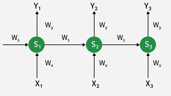
RNN Architecture
At each timestep t , the RNN maintains a hidden state S_t, that stores information from previous inputs. The hidden state S_t updates by combining the current input X_t and the previous hidden state S_{t-1} , applying an activation function to introduce non-linearity. Then the output Y_t is generated by transforming this hidden state.
S_t = g_1(W_x X_t + W_s S_{t-1})
- S_t represents the hidden state (memory) at time t.
- X_t is the input at time t.
- Y_t is the output at time t.
- W_s, W_x, W_y are weight matrices for hidden states, inputs and outputs, respectively.
Y_t = g_2(W_y S_t)
where g_1 and g_2 are activation functions.
RNN Architecture
Error Function at Time t=3
To train the network, we measure how far the predicted output Y_t is from the desired output d_t using an error function. We use the squared error to measure the difference between the desired output d_t and actual output Y_t:
E_t = (d_t - Y_t)^2
At t=3:
E_3 = (d_3 - Y_3)^2
This error quantifies the difference between the predicted output and the actual output at time 3.
Updating Weights Using BPTT
Backpropagation Through Time (BPTT) updates the weights W_y, W_s, W_x by computing gradients across multiple time steps to minimize error.
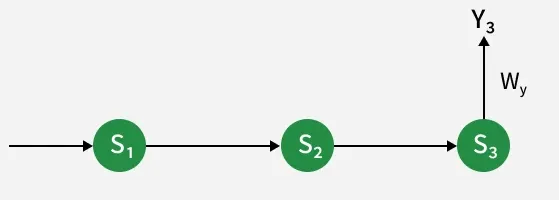
1. Adjusting Output Weight W_y
The output weight W_y directly affects the current output Y_3, so its update depends only on the current time step.
Using the chain rule:
\frac{\partial E_3}{\partial W_y} = \frac{\partial E_3}{\partial Y_3} \times \frac{\partial Y_3}{\partial W_y}
- E_3 depends on Y_3, so we differentiate E_3 w.r.t. Y_3.
- Y_3 depends on W_y, so we differentiate Y_3 w.r.t. W_y.
Adjusting Wy
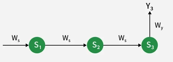
2. Adjusting Hidden State Weight W_s
The hidden state weight W_s affects both the current and previous hidden states because each hidden state depends on the one before it. Therefore, updating W_s, requires considering how all hidden states S_1, S_2, S_3 influence the output at time step 3.
\frac{\partial E_3}{\partial W_s} = \sum_{i=1}^3 \frac{\partial E_3}{\partial Y_3} \times \frac{\partial Y_3}{\partial S_i} \times \frac{\partial S_i}{\partial W_s}
**Gradient Flow Through Hidden States
- Start with the error gradient at output Y_3.
- Propagate gradients back through all hidden states S_3, S_2, S_1 since they affect Y_3.
- Each S_i depends on W_s, so we differentiate accordingly.
Adjusting Ws
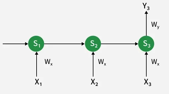
3. Adjusting Input Weight W_x
Similar to W_s, the input weight W_x affects all hidden states because the input at each timestep shapes the hidden state. The process considers how every input in the sequence impacts the hidden states leading to the output at time 3.
\frac{\partial E_3}{\partial W_x} = \sum_{i=1}^3 \frac{\partial E_3}{\partial Y_3} \times \frac{\partial Y_3}{\partial S_i} \times \frac{\partial S_i}{\partial W_x}
The process is similar to W_s, accounting for all previous hidden states because inputs at each timestep affect the hidden states.
Adjusting Wx
Advantages
- Captures temporal dependencies across time steps
- Learns how past inputs influence future outputs
- Forms the foundation for training LSTMs and GRUs
- Supports learning from variable-length sequences
Limitations
- Gradients may become very small (vanishing gradients), making long-term dependencies difficult to learn
- Gradients may grow excessively large (exploding gradients), causing unstable training and updates