SARIMA (Seasonal Autoregressive Integrated Moving Average) (original) (raw)

Last Updated : 7 Apr, 2026

SARIMA or Seasonal Autoregressive Integrated Moving Average is an extension of the traditional ARIMA model, specifically designed for time series data with seasonal patterns. While ARIMA is great for non-seasonal data, SARIMA introduces seasonal components to handle periodic fluctuations and provides better forecasting capabilities for seasonal data.

Understanding the Components of SARIMA

SARIMA consists of several components that help capture both short-term and long-term dependencies within a time series:

**Seasonal Component: Represents the repeating patterns or cycles in the data at regular intervals like yearly, monthly, daily, etc. This allows SARIMA to model seasonality effectively.
**Autoregressive (AR) Component: Models the relationship between current and past observations. It captures the autocorrelation of the data over time.
**Integrated (I) Component: Addresses non-stationarity by differencing the data to make it stationary which is crucial for time series analysis.
**Moving Average (MA) Component: Models the relationship between current observations and past residual errors. It helps in capturing short-term fluctuations.

SARIMA Notation

The SARIMA model is represented as:

**SARIMA(p, d, q)(P, D, Q, s)

**Parameters:

**p: Autoregressive order
**d: Number of non-seasonal differences
**q: Moving average order
**P: Seasonal autoregressive order
**D: Seasonal differencing order
**Q: Seasonal moving average order
**s: Length of the seasonal period (e.g., 12 for monthly data)

Before applying SARIMA, seasonal differencing is often required to make the data stationary. This process involves subtracting the current observation from one that corresponds to the same season in the previous cycle. Seasonal differencing helps remove the seasonal pattern from the data, enabling more accurate forecasting.

Understanding Mathematical Representation of SARIMA

The SARIMA model can be expressed mathematically as:

(1 - \phi_1 B) (1 - \Phi_1 B^s) (1 - B) (1 - B^s) y_t = (1 + \theta_1 B) (1 + \Theta_1 B^s) \epsilon_t

**Parameters:

y_t: The observed time series at time t
B: The backshift operator (lag operator)
\phi_1: Non-seasonal autoregressive coefficient
\Phi_1: Seasonal autoregressive coefficient
\theta_1: Non-seasonal moving average coefficient
\Theta_1: Seasonal moving average coefficient
s: Seasonal period
\epsilon_t: The white noise error term

Implementing SARIMA in Time Series Forecasting

1. Importing Libraries

To begin working with SARIMA, we need to import the necessary libraries like Numpy, Pandas, Matplotlib, Statsmodels and Scikit-learn.

Python `

import numpy as np import pandas as pd import matplotlib.pyplot as plt from statsmodels.tsa.statespace.sarimax import SARIMAX from statsmodels.tsa.stattools import adfuller from statsmodels.graphics.tsaplots import plot_acf, plot_pacf from sklearn.metrics import mean_absolute_error, mean_squared_error

2. Loading the Dataset

We will load a retail dataset to predict monthly sales for a global superstore.

You can download dataset from here.

**pd.read_csv(): Reads the CSV file into a DataFrame.
**df[['Order Date', 'Sales']]: Selects relevant columns ('Order Date' and 'Sales') for analysis.
**pd.to_datetime(): Converts 'Order Date' to datetime format for proper time series analysis. Python `

df = pd.read_csv("/content/Dataset- Superstore (2015-2018).csv") sales_data = df[['Order Date', 'Sales']]

sales_data['Order Date'] = pd.to_datetime(sales_data['Order Date']) sales_data.head()

**Output:

data

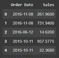
Dataset

We will aggregate the data on a monthly basis to focus on trends rather than daily fluctuations.

**set_index('Order Date'): Sets 'Order Date' as the index of the DataFrame.
**resample('ME').sum(): Resamples the data to monthly frequency and calculates the total sum of sales for each month. Python `

df1 = sales_data.set_index('Order Date') monthly_sales = df1.resample('ME').sum() monthly_sales.head()

**Output:

monthly_data

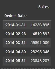
Monthly Sales

4. Plotting the Monthly Sales

Visualizing the sales data helps us identify seasonal patterns.

**plt.figure(figsize=(10, 6)): Sets the plot size.
**plt.plot(): Plots the data with specified line width and color.
**plt.title(), plt.xlabel(), plt.ylabel(): Adds title and labels to the plot.
**plt.show(): Displays the plot. Python `

plt.figure(figsize=(10, 6)) plt.plot(monthly_sales['Sales'], linewidth=3, c='deeppink') plt.title("Monthly Sales") plt.xlabel("Date") plt.ylabel("Sales") plt.show()

**Output:

month_plot

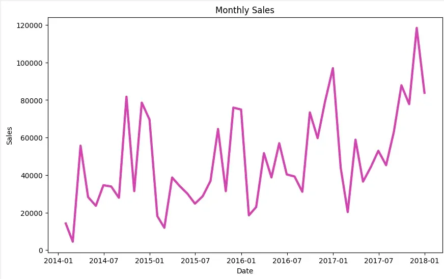
Plotting Monthly Sales

5. Stationarity Check

Before applying SARIMA, we need to check if the data is stationary. Stationary data has constant mean and variance, which is a key assumption for SARIMA. We use the Augmented Dickey-Fuller test (ADF) for this.

**adfuller(timeseries, autolag='AIC'): Performs the Augmented Dickey-Fuller test for stationarity.
**result[1]: Extracts the p-value from the ADF test to check for stationarity.
**result[0]: Displays the ADF statistic. Python `

def check_stationarity(timeseries): result = adfuller(timeseries, autolag='AIC') p_value = result[1] print(f'ADF Statistic: {result[0]}') print(f'p-value: {p_value}') print('Stationary' if p_value < 0.05 else 'Non-Stationary')

check_stationarity(monthly_sales['Sales'])

**Output:

ADF Statistic: -4.493767844002665
p-value: 0.00020180198458237758
Stationary

6. Identifying Model Parameters

We can identify the SARIMA model parameters (p, d, q, P, D, Q, s) using Autocorrelation (ACF) and Partial Autocorrelation (PACF) plots. These plots help in determining the order of the model components.

**plot_acf(): Plots the Autocorrelation Function (ACF) to visualize correlations between lags.
**plot_pacf(): Plots the Partial AutoCorrelation Function (PACF) to visualize partial correlations between lags. Python `

plot_acf(monthly_sales) plot_pacf(monthly_sales) plt.show()

**Output:

acf

ACF

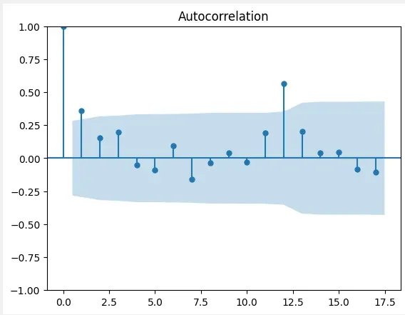
pacf

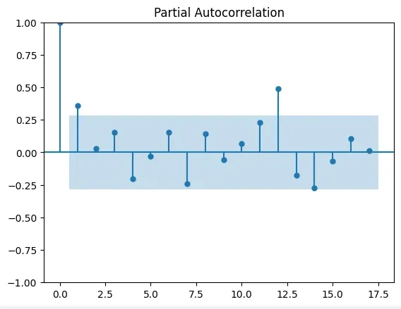
PACF

7. Fitting the SARIMA Model

Once we have identified the model parameters, we can fit the SARIMA model using the SARIMAX function.

**SARIMAX(): Initializes the SARIMA model with specified non-seasonal and seasonal parameters.
**fit(): Fits the SARIMA model to the historical data. Python `

p, d, q = 1, 1, 1 P, D, Q, s = 1, 1, 1, 12

model = SARIMAX(monthly_sales, order=(p, d, q), seasonal_order=(P, D, Q, s)) results = model.fit()

8. Generating Forecasts

With the SARIMA model fitted, we can forecast future sales values. For example, forecasting the next 12 months.

**result.forecast(steps=forecast_periods): Generates the forecast for future time steps.
**plt.plot(): Plots the observed and forecasted data.
**plt.legend(): Adds a legend to the plot to label observed and forecasted data. Python `

forecast_periods = 12 forecast = results.forecast(steps=forecast_periods)

plt.figure(figsize=(10, 6)) plt.plot(monthly_sales, label='Observed') plt.plot(forecast, label='Forecast', color='red') plt.title("Sales Forecast") plt.xlabel("Date") plt.ylabel("Sales") plt.legend() plt.show()

**Output:

forecast

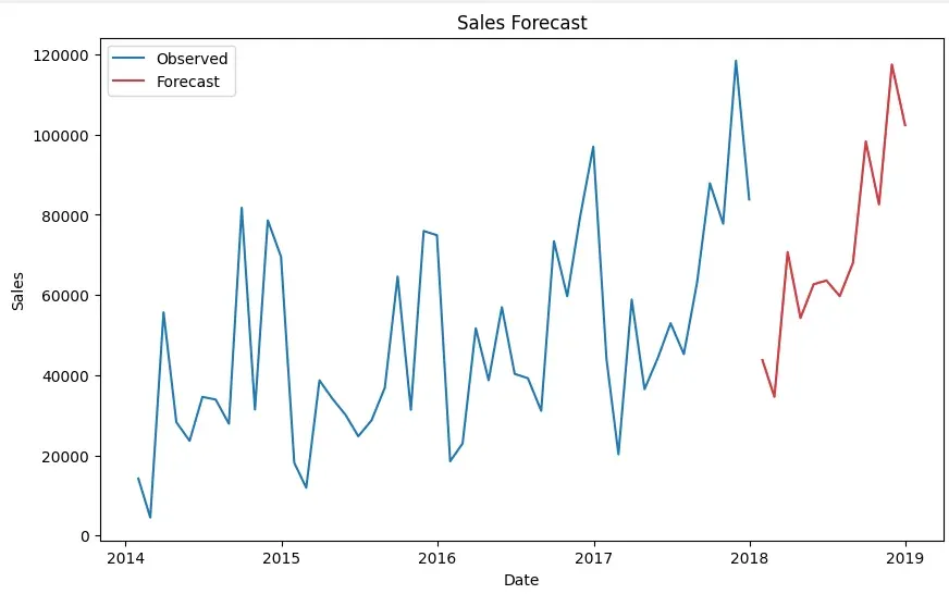
Forecasts

9. Evaluating the Model

We evaluate the model’s forecast accuracy using Mean Absolute Error (MAE) and Mean Squared Error (MSE).

**mean_absolute_error(): Computes the Mean Absolute Error (MAE) to measure prediction accuracy.
**mean_squared_error(): Computes the Mean Squared Error (MSE) to assess model performance. Python `

Take last 12 months as observed values

observed = monthly_sales.tail(forecast_periods)

mae = mean_absolute_error(observed, forecast) mse = mean_squared_error(observed, forecast)

print("MAE:", mae) print("MSE:", mse)

**Output:

MAE: 10611.591984026598
MSE: 151953342.15188608

You can download source code from here.