Stochastic Gradient Descent In R (original) (raw)
Last Updated : 30 Apr, 2026
Stochastic Gradient Descent (SGD) is an optimization algorithm used in machine learning to minimize a model loss function by iteratively updating its parameters. Instead of computing gradients using the entire dataset, SGD updates model weights using a single randomly selected data point or a small batch which makes the training process faster and more scalable.
- Updates parameters using one sample (or a small batch), reducing computation required in each iteration and making it suitable for large datasets.
- Frequent parameter updates allow the model to learn faster and explore the parameter space more effectively.
- Commonly used in training neural networks where weights and biases are updated iteratively to minimize the loss function.
- Introduces randomness during training, which can help the model escape local minima and improve generalization.

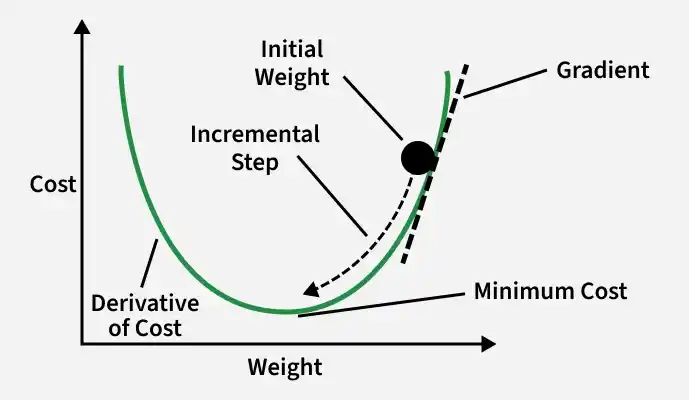
Path followed by batch gradient descent vs. path followed by SGD
Here in above image Gradient Descent follows a smooth and direct path toward the minimum, SGD takes a noisier and zig-zag path due to updates based on individual data samples.
Working
Stochastic Gradient Descent (SGD) minimizes a loss function by iteratively updating model parameters using the gradient computed from a randomly selected training example. SGD performs updates after evaluating a single data point or a small mini-batch.
SGD Working
1. Objective Function
The goal of SGD is to minimize the loss function, which measures how far the model’s prediction is from the actual value.. The objective function defined as:
J(\theta) = \frac{1}{n} \sum_{i=1}^{n} L(y_i, \hat{y}_i)
where
- n: total number of training samples
- y_{i}: actual value
- \hat{y}_i: predicted value
- L: loss function
2. Gradient Calculation
To reduce the loss, we calculate the gradient, which tells us how much the parameters should change.
\text{Gradient} = \frac{\partial L}{\partial w}
where
- \partial represents the partial derivative.
- w represents the model weight (parameter).
- \frac{\partial L}{\partial w} represents how the loss changes with respect to the weight.
3. Parameter Update Rule
Once the gradient is calculated, the model parameters are updated using the SGD update rule:
w = w - \eta \times \text{Gradient}
where \eta is learning rate.
4. SGD Training Algorithm
The SGD algorithm repeats the following steps until the model converges:
- Initialize the model parameters (weights and bias) with random values and choose a learning rate \eta.
- Randomly shuffle the training dataset to ensure the model learns unbiased patterns.
- Select one training example (x_{i},y_{i}) and compute the predicted output \hat{y}_{i}.
- Calculate the loss and compute the gradient of the loss with respect to the model parameters.
- Update the parameters using the SGD update rule and repeat the process for multiple iterations until the model converges, meaning the loss becomes stable or sufficiently small.
Step By Step Implementation
Here we implement SGD algorithm in R.
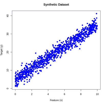
Step 1: Generate and Visualize Synthetic Dataset
Here we create a synthetic dataset with a linear relationship between x and y and add random noise. A scatter plot is used to visualize the data distribution.
R `
set.seed(42)
n <- 1000
x <- runif(n, 0, 10)
y <- 3*x + 5 + rnorm(n, 0, 2)
data <- data.frame(x, y)
plot(x, y, main="Synthetic Dataset", xlab="Feature (x)", ylab="Target (y)", pch=19, col="blue")
`
**Output:
Output
Step 2: Initialize Model Parameters and Training Settings
We randomly initialize the model weight and bias, set the learning rate, define the number of training epochs and create a vector to store the loss at each epoch.
R `
w <- runif(1)
b <- runif(1)
learning_rate <- 0.01
epochs <- 500
loss_history <- c()
`
Step 3: Train Model Using Stochastic Gradient Descent
Here we train the linear regression model by updating the weight and bias for each training example. The dataset is shuffled every epoch and the loss is recorded to track training progress.
R `
for (epoch in 1:epochs) { data <- data[sample(nrow(data)),] for (i in 1:nrow(data)) {
xi <- data$x[i]
yi <- data$y[i]
y_pred <- w*xi + b
error <- y_pred - yi
dw <- 2 * error * xi
db <- 2 * error

w <- w - learning_rate * dw
b <- b - learning_rate * db
}
predictions <- w*data$x + b loss <- mean((data$y - predictions)^2) loss_history <- c(loss_history, loss) }
`
Step 4: Display Final Model Parameters
After training, we print the final weight and bias learned by the model to see the values that best fit the dataset.
R `
cat("Final Weight:", w, "\n") cat("Final Bias:", b, "\n")
`
**Output:
Final Weight: 3.3142
Final Bias: 4.718445
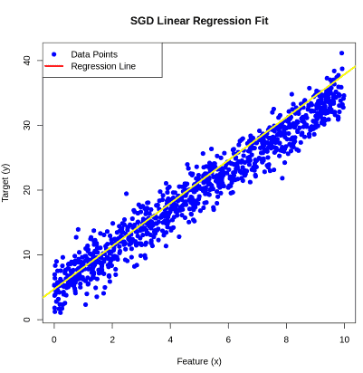
Step 5: Visualize Regression Line
Plot the training data points and draw the regression line using the final weight and bias learned by SGD to see how well the model fits the data.
R `
plot(x, y, main="SGD Linear Regression Fit", xlab="Feature (x)", ylab="Target (y)", pch=19, col="blue")
abline(a=b, b=w, col="yellow", lwd=3)
legend("topleft", legend=c("Data Points","Regression Line"), col=c("blue","yellow"), pch=c(19,NA), lwd=c(NA,3))
`
**Output:
Output
Hyperparameters in SGD
The performance and convergence of Stochastic Gradient Descent (SGD) depend on the choice of its hyperparameters. Choosing the right values for these parameters is critical for efficient training and achieving optimal model performance.
1. Learning Rate
The learning rate (\eta) controls the step size the algorithm takes towards minimizing the loss function. It is one of the most sensitive hyperparameters in SGD.
- **Too High: The algorithm may overshoot the minimum or diverge entirely.
- **Too Low: Convergence becomes very slow and the model may get stuck in local minima.
- **Strategy: Start with a small value such as 0.01. You can also use learning rate schedules or adaptive learning rate methods (like Adam or RMSProp) to adjust it dynamically during training.
2. Batch Size
The batch size determines how many data points are used to compute the gradient in each update step.
- **Stochastic (Batch Size = 1): Each update uses a single data point, introducing more noise but enabling faster iterations.
- **Mini-Batch: Balances computational efficiency and noise, making it the most commonly used approach in practice.
- **Full Batch: Uses the entire dataset for each update. This reduces gradient noise but increases computation time per iteration.
- **Strategy: Mini-batches are preferred for large datasets. Using smaller batches can also act as a regularizer due to the inherent noise in gradient estimation.
3. Epochs
An epoch is a complete pass through the entire dataset. The number of epochs determines how many times the model sees the data during training.
- **Too Few Epochs: The model may underfit, failing to capture patterns in the data.
- **Too Many Epochs: The model may overfit, learning noise rather than meaningful patterns.
- ****Strategy:**Start with 100–500 epochs and monitor the loss or validation performance. Early stopping can be applied to halt training when performance stops improving.
Let’s consider a dataset where we want to perform Hyperparameters on Stochastic Gradient Descent In R.
Step 1:Load Necessary Libraries and Generate Synthetic Data
This step installs and loads the required library (ggplot2) and generates a synthetic 2D dataset for logistic regression.
R `
if (!requireNamespace("ggplot2", quietly = TRUE)) install.packages("ggplot2") library(ggplot2)
set.seed(42)
n <- 100 x1 <- runif(n, min = -10, max = 10) x2 <- runif(n, min = -10, max = 10) y <- ifelse(x1 + x2 + rnorm(n) > 0, 1, 0)
data <- data.frame(x1 = x1, x2 = x2, y = y)
ggplot(data, aes(x = x1, y = x2, color = factor(y))) + geom_point() + labs(title = "Synthetic Data for Logistic Regression", x = "x1", y = "x2", color = "Class") + theme_minimal()
`
**Output:
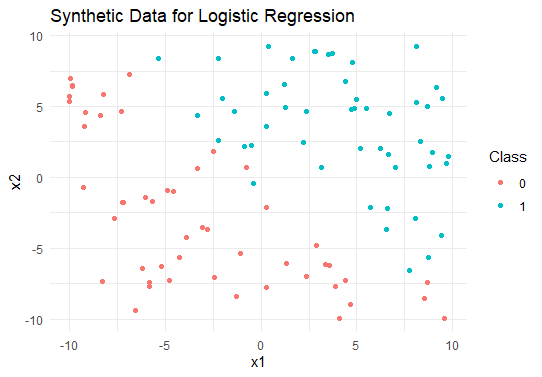
Synthetic Data for Logistic Regression
Step 2: Define the Logistic Function
The logistic function converts linear outputs into probabilities between 0 and 1.
R `
Logistic function
logistic <- function(z) { return(1 / (1 + exp(-z))) }
`
Step 3: Compute Gradients
This function calculates the gradient of the loss for a single sample to update weights and bias.
R `
compute_loss_and_gradient <- function(x1, x2, y, w, b) { z <- w[1] * x1 + w[2] * x2 + b predictions <- logistic(z) error <- predictions - y
grad_w1 <- error * x1 grad_w2 <- error * x2 grad_b <- error
list(grad_w1 = grad_w1, grad_w2 = grad_w2, grad_b = grad_b) }
`
Step 4: Implement SGD for Logistic Regression
Here we trains the logistic regression model using stochastic gradient descent over multiple epochs.
R `
sgd_logistic <- function(data, learning_rate, epochs) { w <- c(0, 0) b <- 0
for (epoch in 1:epochs) { for (i in 1:nrow(data)) { index <- sample(1:nrow(data), 1) x1 <- data$x1[index] x2 <- data$x2[index] y <- data$y[index]
  gradients <- compute_loss_and_gradient(x1, x2, y, w, b)

  w[1] <- w[1] - learning_rate * gradients$grad_w1
  w[2] <- w[2] - learning_rate * gradients$grad_w2
  b    <- b - learning_rate * gradients$grad_b
}
}
list(weights = w, bias = b) }
`
Step 5: Train the Model
Set the learning rate and number of epochs, then train the logistic regression model using SGD.
R `
learning_rate <- 0.01 epochs <- 1000 model <- sgd_logistic(data, learning_rate, epochs) print(model)
`
**Output:
$weights
[1] 1.850376 1.841270
$bias
[1] -0.8065149
Step 6: Visualize Decision Boundary
Plot the synthetic dataset with the decision boundary learned by the logistic regression model.
R `
ggplot(data, aes(x = x1, y = x2, color = factor(y))) + geom_point() + geom_abline(intercept = -model$bias / model$weights[2], slope = -model$weights[1] / model$weights[2], color = "red", linetype = "dashed") + labs(title = "Logistic Regression with SGD", x = "x1", y = "x2", color = "Class") + theme_minimal()
`
**Output:
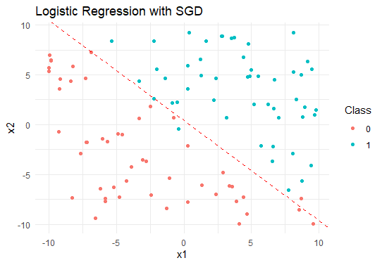
Stochastic Gradient Descent In R
Download full code from here
The output is showing the optimized weights and bias of the logistic regression model and visualize the decision boundary separating the two classes in the plot.
Advantages
- Updates parameters using one sample at a time, making each iteration faster than full batch gradient descent.
- Frequent updates help the model explore the parameter space more effectively, often leading to faster convergence.
- Requires less memory since it processes small batches or single samples, making it suitable for large datasets.
- The randomness in updates helps escape shallow local minima and find better solutions.
- Widely used in deep learning due to its efficiency and scalability.
Limitation
- Random updates introduce noise, causing fluctuations in the loss and less stable convergence.
- Highly sensitive to learning rate; improper values can lead to slow training or divergence.
- May take more epochs to reach the optimal solution due to noisy updates.
- Performs poorly on sparse or unbalanced datasets where single samples may not represent overall patterns.
- Without enhancements like momentum or adaptive methods, it may struggle with complex loss surfaces.