LSTM Networks (original) (raw)
Last Updated : 5 Jan, 2026
Long Short-Term Memory (LSTM) networks are a special type of recurrent neural network designed to learn from sequence data while overcoming the limitations of traditional RNNs. With their unique memory‑cell structure, LSTMs can remember information over long time intervals, making them highly effective for tasks involving patterns across time.
- Handles long‑term dependencies without vanishing gradients
- Uses gates to control how information is stored and forgotten
- Widely used in NLP, time‑series forecasting and speech processing
- Performs well on sequential and temporal prediction problems
Working of LSTM
Let's understand the working:
Step 1: Decide What to Forget (Forget Gate)
- The forget gate takes the previous hidden state h_{t-1} and the current input x_t.
- It produces values between 0 and 1 using a sigmoid activation.
- These values determine how much of the previous cell state C_{t-1} should be kept.
- Values near 1 mean the information is retained.
- Values near 0 mean the information is discarded.
- This mechanism helps remove outdated or irrelevant context from long sequences.
Step 2: Decide What New Information to Add (Input Gate + Candidate Memory)
- The input gate determines how much of the new information should be written into the memory.
- The candidate memory creates a new vector of potential information using a tanh activation.
- The input gate filters the candidate memory before it is added to the cell state.
- This ensures that only relevant new information updates the internal memory.
Step 3: Update the Cell State (Memory Highway)
- The updated cell state is formed by combining the scaled previous memory and the filtered new memory.
- The forget gate reduces or removes parts of the old memory.
- The input gate and candidate memory add new information to fill in or modify the cell state.
- Additive updates help gradients flow more consistently, preventing the vanishing gradient problem.
- This stable memory path enables learning complex long-range patterns.
Step 4: Generate the Output (Output Gate)
- The output gate determines how much of the updated cell state influences the hidden state h_t .
- A sigmoid activation computes this output filter.
- The filtered value is merged with the tanh-transformed cell state to produce the final hidden state.
- The hidden state serves as the LSTM’s output at time step t.
- The same hidden state is passed forward to the next time step for continued processing.
Step-By-Step Implementation
Here build an LSTM-based deep learning model to predict IBM stock prices using historical data.
The used dataset can be downloaded from here.
Step 1: Import Required Libraries
- Import NumPy, Pandas and Matplotlib for numerical operations, data processing and plotting stock prices.
- MinMaxScaler normalizes data.
- Keras is used to build the deep learning model.
- mean_squared_error and math are used to calculate prediction performance metrics like RMSE. Python `
import math from sklearn.metrics import mean_squared_error from keras.layers import LSTM, Dense, Dropout from keras.models import Sequential from sklearn.preprocessing import MinMaxScaler import pandas as pd import numpy as np import matplotlib.pyplot as plt plt.style.use('fivethirtyeight')
def plot_predictions(real_prices, predicted_prices): plt.figure(figsize=(16, 6)) plt.plot(real_prices, color='green', label='Actual IBM Stock Price') plt.plot(predicted_prices, color='orange', label='Predicted IBM Stock Price') plt.title('IBM Stock Price Prediction') plt.xlabel('Time') plt.ylabel('Stock Price') plt.legend() plt.show()
def calculate_rmse(real_prices, predicted_prices): rmse = math.sqrt(mean_squared_error(real_prices, predicted_prices)) print(f"Root Mean Squared Error (RMSE): {rmse:.4f}")
`
Step 2: Load and Visualize IBM Stock Dataset
- Load IBM stock data from a CSV file using read_csv() and set Date as the index for time-series analysis.
- Select the High price column as the target feature for prediction.
- Split data into Training and Testing sets. Python `
dataset = pd.read_csv("IBM_2006-01-01_to_2018-01-01.csv", index_col='Date', parse_dates=['Date'])
training_set = dataset.loc[:'2016', 'High'].values.reshape(-1, 1) test_set = dataset.loc['2017':, 'High'].values.reshape(-1, 1)
plt.figure(figsize=(16, 4)) plt.plot(dataset.loc[:'2016', 'High'], label='Training Set (Before 2017)') plt.plot(dataset.loc['2017':, 'High'], label='Test Set (2017 and beyond)') plt.title('IBM Stock Price') plt.xlabel('Date') plt.ylabel('Price') plt.legend() plt.show()
`
**Output:
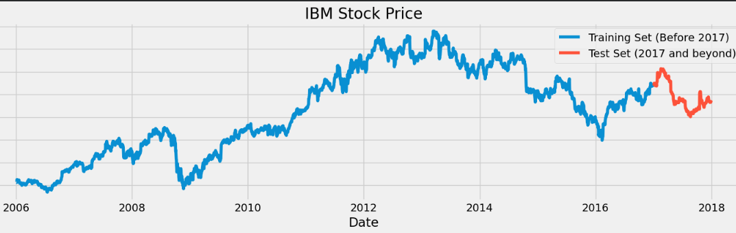
IBM stock data
Step 3: Apply Feature Scaling
- LSTM models require normalized values to learn effectively and improve convergence.
- Apply MinMaxScaler to scale stock prices between 0 and 1.
- Normalization prevents issues like gradient explosion or vanishing during training.
- Scaling makes the training process more stable, faster and accurate. Python `
scaler = MinMaxScaler(feature_range=(0, 1)) scaled_training = scaler.fit_transform(training_set)
`
Step 4: Prepare Training Sequences
- LSTMs require fixed length time series sequences for learning patterns over time.
- Use the previous 60 days of stock prices to predict the next day value.
- Create X_train with 60 timestep inputs and Y_train with the next-day output.
- Reshape input to 3D format for LSTM compatibility. Python `
X_train = [] y_train = []
for i in range(60, len(scaled_training)): X_train.append(scaled_training[i - 60:i, 0]) y_train.append(scaled_training[i, 0])
X_train = np.array(X_train) y_train = np.array(y_train)
X_train = X_train.reshape(X_train.shape[0], X_train.shape[1], 1)
`
Step 5: Build the LSTM Model
- Build a stacked LSTM architecture with four layers containing 50 units each to learn deep time dependencies.
- Add Dropout after every LSTM layer to reduce overfitting and improve generalization.
- Use a Dense layer to output the final predicted stock price value.
- Compile the model using RMSProp optimizer and Mean Squared Error (MSE) loss function. Python `
lstm_model = Sequential()
lstm_model.add(LSTM(units=50, return_sequences=True, input_shape=(X_train.shape[1], 1))) lstm_model.add(Dropout(0.2))
lstm_model.add(LSTM(units=50, return_sequences=True)) lstm_model.add(Dropout(0.2))
lstm_model.add(LSTM(units=50, return_sequences=True)) lstm_model.add(Dropout(0.2))
lstm_model.add(LSTM(units=50)) lstm_model.add(Dropout(0.2))
lstm_model.add(Dense(units=1))
lstm_model.compile(optimizer='rmsprop', loss='mean_squared_error')
`
Step 6: Train the Model
- Train the LSTM model for 20 epochs with a batch size of 32 to optimize learning efficiency.
- The model learns historical stock price patterns and trends over time.
- During training, weights are continuously updated to minimize prediction error. Python `
lstm_model.fit(X_train, Y_train, epochs=20, batch_size=32, verbose=1)
`
Step 7: Prepare Test Data for Prediction
- Combine the training and test High prices to create continuous time-series data.
- Take the last 60 days prior to the test period as the input window for prediction.
- Apply the same MinMaxScaler used during training to maintain consistency.
- Generate X_test sequences identical to training format and reshape into 3D structure for LSTM input. Python `
dataset_total = pd.concat( (dataset['High'][:'2016'], dataset['High']['2017':]), axis=0) inputs = dataset_total[len(dataset_total) - len(test_set) - 60:].values inputs = inputs.reshape(-1, 1) inputs = scaler.transform(inputs)
X_test = [] for i in range(60, len(inputs)): X_test.append(inputs[i - 60:i, 0])
X_test = np.array(X_test) X_test = X_test.reshape(X_test.shape[0], X_test.shape[1], 1)
`
Step 8: Predict Stock Prices
- Use the trained LSTM model to generate scaled predictions on test input sequences.
- Apply inverse_transform() to convert predictions back to original price values.
- The output represents the final predicted IBM stock prices.
- These values can now be compared with actual prices for evaluation. Python `
predicted_prices_scaled = lstm_model.predict(X_test) predicted_prices = scaler.inverse_transform(predicted_prices_scaled)
`
Step 9: Plot Actual vs Predicted Prices
- Plot the actual vs predicted IBM stock prices for visual performance evaluation.
- Helps check how closely LSTM predictions follow real market trends.
- Visualization highlights how well patterns and price movements are learned. Python `
plot_predictions(test_set, predicted_prices)
`
**Output:
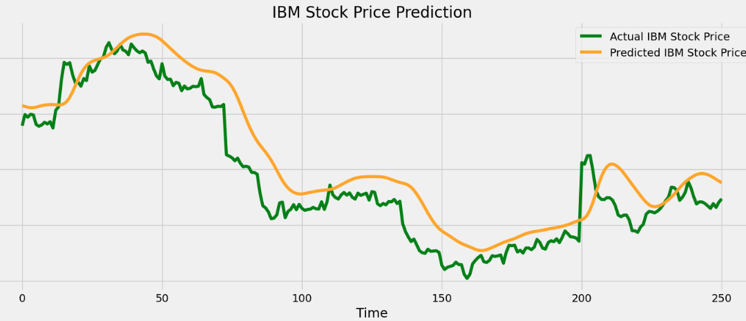
Stock Price Prediction
As we can see our model is working fine and is doing accurate predictions.
You can download full code from here
LSTM Variations
1. Vanilla LSTM (Standard LSTM)
- This is the basic version of the LSTM architecture containing a single LSTM layer.
- It processes the input sequence step-by-step using its memory cell and gating system.
- It is suitable for tasks where patterns are not overly complex or hierarchical.
- It serves as the foundation for more advanced LSTM architectures.
2. Stacked LSTM (Deep LSTM)
- Multiple LSTM layers are placed on top of each other, allowing deeper sequence representation learning.
- Lower layers learn simple temporal patterns, while higher layers capture more abstract relationships.
- This architecture is helpful when the task involves complex dependencies across multiple sequence levels.
- It is commonly used in deep learning tasks such as speech modeling and advanced NLP problems.
3. Bidirectional LSTM (BiLSTM)
- The sequence is processed in both forward and backward directions.
- This allows the model to understand both past and future context for each time step.
- It improves performance in tasks where understanding full surrounding context is important such as sentiment analysis and named entity recognition.
- It is especially useful in text-based tasks where each word’s meaning depends on both previous and next words.
4. Peephole LSTM
- Gates are allowed to directly access the cell state, improving timing precision.
- This variation enhances performance in tasks that require fine control of memory updates, such as modeling periodic or time-sensitive patterns.
- It gives the model more visibility into the internal memory dynamics during gate decisions.
5. CNN–LSTM Hybrid
- Convolutional layers handle spatial feature extraction, while LSTMs capture temporal dynamics.
- This combination is useful for sequential image tasks, video analysis and sensor signal recognition.
- CNN layers reduce input dimensionality, allowing LSTMs to focus on temporal relationships more efficiently.
6. Encoder–Decoder LSTM
- One LSTM acts as an encoder to compress the sequence into a fixed representation.
- Another LSTM acts as a decoder to generate the output sequence.
- This structure is used in tasks like machine translation, text summarization and sequence generation.
- It was the main architecture for seq-to-seq models before attention and transformer mechanisms became popular.
7. Attention-LSTM Models
- Attention mechanisms are added to allow the model to focus on specific parts of the input sequence during decoding.
- This significantly improves performance by highlighting important steps rather than treating all equally.
- It is widely used in translation, text generation and speech tasks before full Transformer models took over.
LSTM vs. GRU
Let's compare LSTM and GRU:
| Feature | LSTM | GRU |
|---|---|---|
| Gates | 3 gates (Input, Forget, Output) | 2 gates (Update, Reset) |
| Memory Structure | Separate Cell State + Hidden State | Single combined Hidden State |
| Complexity | More complex, more parameters | Simpler, fewer parameters |
| Training Speed | Slower | Faster |
| Long-Term Dependency Handling | Stronger for very long sequences | Good but slightly less precise for very long dependencies |
| Model Size & Efficiency | Larger and more resource-heavy | Smaller, efficient, suitable for real-time and mobile use |
Applications
- **Natural Language Processing (NLP): They are widely used for tasks like sentiment analysis, text classification and language modeling because they understand long-term word dependencies.
- **Machine Translation: LSTM based encoder–decoder models translate text between languages by learning relationships across long sentence sequences.
- **Speech Recognition: It analyze temporal variations in audio and improve accuracy in converting speech to text.
- **Time-Series Forecasting: It predict future values in financial markets, weather systems, energy demand and other temporal datasets.
- **Anomaly Detection: It can detect unusual patterns in sequences, making them useful in fraud detection, network monitoring and industrial fault prediction.