Python Student’s t Distribution in Statistics (original) (raw)
We know the mathematics behind t-distribution. However, we can also use Python to implement t-distribution on a dataset. Python provides a unique package scipy for various statical techniques and methods. We will use this package for t-distribution implementation.
prerequisite: t-distribution
What is t-Distribution
The t-distribution, also known as the Student's t-distribution, is a probability distribution that is used in inferential statistics when the sample size is small and the population standard deviation is unknown. It is a variation of the normal distribution with heavier tails, which makes it more appropriate for estimating the mean of a population when the sample size is small or when there is uncertainty about the population standard deviation.
The t-distribution is characterized by its degrees of freedom (df), which also determines the shape of the t-distribution. The degrees of freedom represent the number of independent features in the dataset. As the degrees of freedom increase, the t-distribution approaches the shape of a standard normal distribution.
Characteristics of t-Distribution
- Symmetry: t-Distribution is symmetric about its mean
- Location and Scale: t-Distribution has generally zero mean however it's standard deviation is greater than zero due to its heavier tail.
- Tails: t-distribution has heavier tails(larger tail) which means there are fewer points closer to the mean as compared to the normal distribution.
- Shape: t-distribution shapes depend upon their degree of freedom. Also, As the degrees of freedom increase, the t-distribution becomes closer to a normal distribution.
The Formula For t-Distribution
the t-distribution looks very similar to normal distribution the only difference is that instead of the standard deviation of the population, we will use the standard deviation of the sample.
t = \frac{\bar{x}-\mu}{\left[\frac{s}{\sqrt{n}}\right]} where, t = The t-score, x̄ = sample mean, μ = population mean, s = standard deviation of the sample, n = sample size
When to Use the t-Distribution
Student’s t Distribution is used when
- The sample size is 30 or less than 30.
- The population standard deviation(σ) is unknown.
- The population distribution must be unimodal and skewed.
Python Implementation of t-Distribution
scipy.stats.t() represents a student’s t continuous random variable. It is inherited from the generic methods as an instance of the rv_continuous class. The rv_continuous class in scipy.stats provides a framework for defining and working with continuous random variables.
Creating Random Values Using Student’s T-distribution
Python3 `
from scipy.stats import t
a, b = 4, 3 rv = t(a, b)
Generate random values from the t-distribution
Replace 10 with the desired number of random values
random_values = rv.rvs(size=5)
print("Random Values: ", random_values)
`
Output :
Random Values: [3.46225158 2.68564689 2.81650105 1.26304106 3.9418692 ]
By calling t(a, b), Here we are creating an instance of the Student's t continuous random variable with the specified parameters a (degrees of freedom) and b (location parameter). The resulting variable rv is then used for generating five(size=5) random values.
Student’s T-Distribution Continuous Variates and Probability Distribution
We will create a random variate from t-distribution having a degree of freedom at the b location parameter. Then we will find the probability distribution of the random variate at the quantile that we have created using numpy.
Python3 `
import numpy as np quantile = np.arange(0.01, 1, 0.1)
Random Variates
R = t.rvs(a, b) print("Random Variates : ", R)
R = t.pdf(a, b, quantile) print("Probability Distribution : ", R)
`
Output :
Random Variates : 2.877894570989561
Probability Distribution : [0.00663446 0.00721217 0.0078511 0.00855881 0.00934388 0.01021611 0.01118667 0.01226833 0.01347568 0.01482539]
Graphical Representation of Random Values Created Using T-Distribution.
Python3 `
import numpy as np import matplotlib.pyplot as plt
distribution = np.linspace(0, np.minimum(rv.dist.b, 3)) print("Distribution: , distribution)
plot = plt.plot(distribution, rv.pdf(distribution))
`
Output :
Distribution : [0.0.04081633 0.08163265 0.12244898 0.16326531 0.20408163 0.24489796 0.28571429 0.32653061 0.36734694 0.40816327 0.44897959 0.48979592 0.53061224 0.57142857 0.6122449 0.65306122 0.69387755 0.73469388 0.7755102 0.81632653 0.85714286 0.89795918 0.93877551 0.97959184 1.02040816 1.06122449 1.10204082 1.14285714 1.18367347 1.2244898 1.26530612 1.30612245 1.34693878 1.3877551 1.42857143 1.46938776 1.51020408 1.55102041 1.59183673 1.63265306 1.67346939 1.71428571 1.75510204 1.79591837 1.83673469 1.87755102 1.91836735 1.95918367 2.]
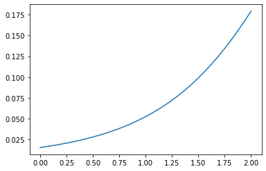
T-distribution graph
T-Distribution Graph With Varying Positional Arguments
If we change the location parameter of T-Distribution then the position of the graph shifts itself
Python3 `
import matplotlib.pyplot as plt import numpy as np
x = np.linspace(0, 5, 100)
Varying positional arguments
y1 = t.pdf(x, 1, 3) y2 = t.pdf(x, 1, 4) plt.plot(x, y1, "*", x, y2, "r--") plt.show()
`
Output:
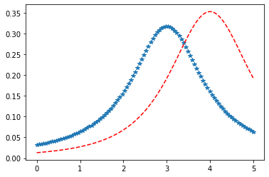
T-distribution graph with varying positional argument
T-Distribution Graph With Varying Degrees of Freedom
With the change in the degree of freedom of the t-distribution with fixed location parameter number of points located at mean changes (height of t-distribution changes).
Python3 `
import matplotlib.pyplot as plt import numpy as np from scipy.stats import t
x = np.linspace(-5, 5, 100) degrees_of_freedom = [1, 2, 5, 10] # Varying degrees of freedom
Plotting T-distribution curves for different degrees of freedom
for df in degrees_of_freedom: y = t.pdf(x, df) # Using default location and scale parameters (0 and 1) plt.plot(x, y, label=f"Degrees of Freedom = {df}")
plt.xlabel('x') plt.ylabel('PDF') plt.title('T-Distribution with Varying Degrees of Freedom') plt.legend() plt.show()
`