Python | Visualize graphs generated in NetworkX using Matplotlib (original) (raw)
**NetworkX is a Python library used to create and analyze graph structures. Although it's mainly for graph analysis, it also offers basic tools to visualize graphs using Matplotlib. In this article, you'll learn how to draw, label and save graphs using NetworkX's built-in drawing functions.
Steps to Visualize a Graph in NetworkX
1. Import the required libraries
import networkx as nx
import matplotlib.pyplot as plt
2. Generate a graph using networkx.Graph() or another graph class like DiGraph, MultiGraph, etc.
g.add_edge(1, 2)
3. Add edges (or nodes) to the graph using methods such as:
g.add_edge(1, 2)
4. Draw the graph using:
nx.draw(g)
5. (Optional) Add node labels using:
nx.draw(g, with_labels=True)
6. Save the plot as an image file using:
plt.savefig("filename.png")
Basic Example: Draw and Save a Graph
Python `
import networkx as nx import matplotlib.pyplot as plt
g = nx.Graph()
g.add_edge(1, 2) g.add_edge(2, 3) g.add_edge(3, 4) g.add_edge(1, 4) g.add_edge(1, 5)
nx.draw(g) plt.savefig("filename.png")
`
**Output
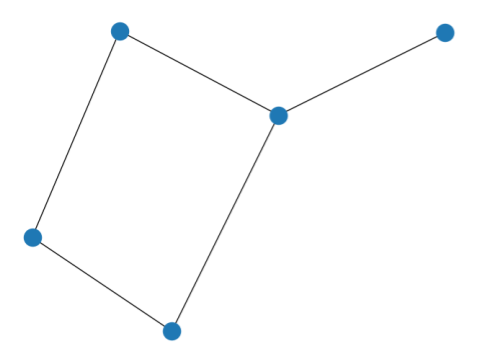
**Explanation: This code creates a simple undirected graph with 5 nodes and 5 edges, draws it and saves the output as **filename.png.
Adding Node Labels
To include numbers (or labels) on nodes, simply set with_labels=True:
Python `
import networkx as nx import matplotlib.pyplot as plt
g = nx.Graph()
g.add_edge(1, 2) g.add_edge(2, 3) g.add_edge(3, 4) g.add_edge(1, 4) g.add_edge(1, 5)
nx.draw(g, with_labels=True) plt.savefig("filename.png")
`
**Output:
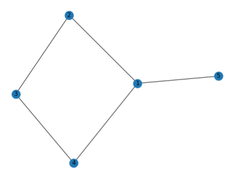
**Explanation: Here, **with_labels=True displays the node numbers in the graph, making it easier to understand connections.
Custom Layouts for Graph Drawing
NetworkX provides several graph layout algorithms to control how the graph is visually arranged. You can use various draw_* functions to apply different layouts:
| Layout | Function Used | Description |
|---|---|---|
| Circular | nx.draw_circular() | Arranges nodes in a circle |
| Planar | nx.draw_planar() | For planar graphs (no edge crossings) |
| Random | nx.draw_random() | Places nodes randomly |
| Spectral | nx.draw_spectral() | Based on eigenvectors of the graph Laplacian |
| Spring | nx.draw_spring() | Uses Fruchterman-Reingold force-directed algorithm |
| Shell | nx.draw_shell() | Arranges nodes in concentric circles |
Example with All Layouts
Python `
import networkx as nx import matplotlib.pyplot as plt
g = nx.Graph()
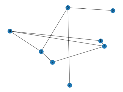
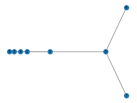
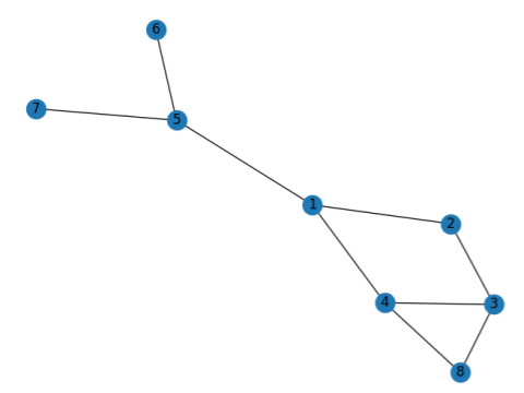
g.add_edge(1, 2) g.add_edge(2, 3) g.add_edge(3, 4) g.add_edge(1, 4) g.add_edge(1, 5) g.add_edge(5, 6) g.add_edge(5, 7) g.add_edge(4, 8) g.add_edge(3, 8)
Circular Layout
nx.draw_circular(g, with_labels=True) plt.savefig("filename1.png") plt.clf()
Planar Layout
nx.draw_planar(g, with_labels=True) plt.savefig("filename2.png") plt.clf()
Random Layout
nx.draw_random(g, with_labels=True) plt.savefig("filename3.png") plt.clf()
Spectral Layout
nx.draw_spectral(g, with_labels=True) plt.savefig("filename4.png") plt.clf()
Spring Layout
nx.draw_spring(g, with_labels=True) plt.savefig("filename5.png") plt.clf()
Shell Layout
nx.draw_shell(g, with_labels=True) plt.savefig("filename6.png") plt.clf()
`
**Circular Layout
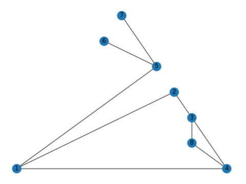
**Planar Layout
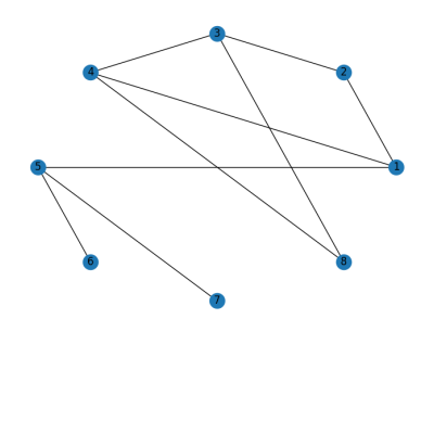
**Random Layout
**Spectral Layout
**Spring Layout
**Shell Layout
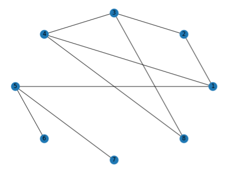
**Explanation: A simple undirected graph is created using networkx.Graph() with added edges to define connections. The graph is visualized using six different NetworkX layouts, each saved as a separate image:
- **nx.draw_circular() arranges nodes evenly in a circle, ideal for symmetrical or cyclic graphs.
- **nx.draw_planar() tries to avoid edge crossings, working only for planar graphs.
- **nx.draw_random() places nodes arbitrarily, offering quick but unstructured visuals.
- **nx.draw_spectral() uses graph Laplacian eigenvalues to highlight structural patterns.
- **nx.draw_spring() simulates nodes as repelling bodies with spring-like edges for a balanced look.
- **nx.draw_shell() positions nodes in concentric circles, useful for layered or hierarchical data.