Clustering in R Programming (original) (raw)

Last Updated : 14 Apr, 2026

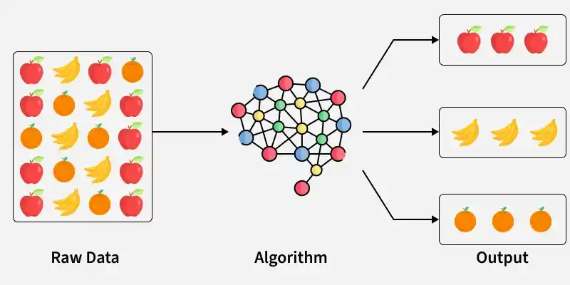
Clustering is an unsupervised learning technique that organizes data points into groups based on their similarity. It reveals underlying patterns, structures and relationships within a dataset without the need for labeled data.

• Groups data points so that those within the same cluster are more similar to each other than to points in other clusters.
• Helps detect hidden patterns, natural groupings and behavior trends in data.
• Useful for dimensionality reduction, anomaly detection and as a preprocessing step for supervised learning tasks.

Clustering

Here unstructured data is processed by a clustering algorithm to automatically group similar items into meaningful clusters in the output.

**Clustering Algorithms in R Programming

In R, there are different clustering techniques that work with various types of data and address specific clustering challenges. Each method has its own strengths and can handle aspects like the number of clusters, their shapes and the presence of noise in the data.

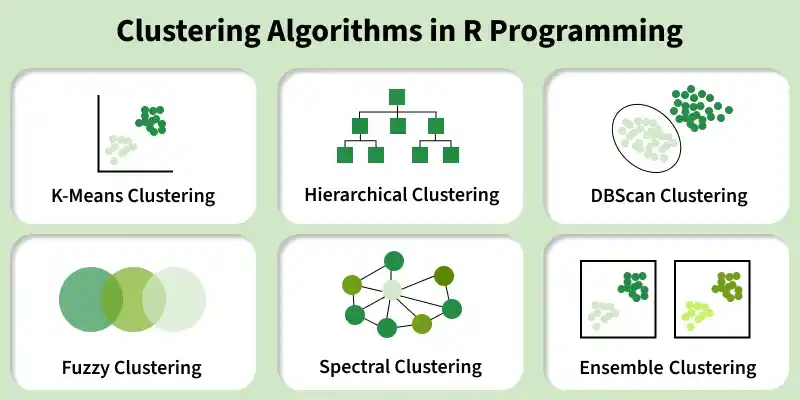
Clustering Algorithms

1. K-Means Clustering

K-Means clustering is a widely used unsupervised learning algorithm that groups data points into a specified number of clusters based on their features. It works by iteratively assigning points to the nearest cluster center and updating the cluster centroids until convergence. K-Means is simple, fast and effective for many real-world datasets.

**Implementation: Here we apply K-Means clustering on the mtcars dataset and visualizes the resulting clusters using the factoextra package.

• The dataset is prepared by removing missing values and scaling all features so that each variable contributes equally to the clustering.
• K-Means clustering is applied with 4 clusters, using multiple random starts to ensure stable and reliable results. R `

install.packages("factoextra") library(factoextra)

df <- mtcars df <- na.omit(df)
df_scaled <- scale(df)

set.seed(123)

km4 <- kmeans(df_scaled, centers = 4, nstart = 25)

fviz_cluster(km4, data = df_scaled, geom = "point", ellipse.type = "convex", main = "K-Means Clustering (k=4)")

`

**Output:

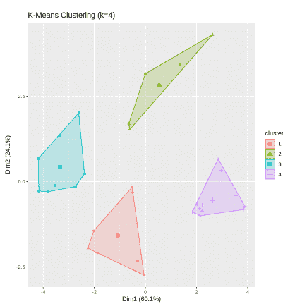
K means Clustering

2. Hierarchical Clustering

Hierarchical Clustering is an unsupervised learning method that groups data points into a tree-like structure based on their similarity. Instead of specifying the number of clusters in advance, it builds a hierarchy of clusters that can be visualized using a dendrogram. This method is useful when you want to understand the relationships between data points at different levels of similarity.

**Implementation: Here we implement Hierarchical Clustering on the Wholesale Customers dataset and visualizes the resulting clusters.

Download dataset from here

• Load the dataset, select numerical features and standardize the data using scale() for proper clustering.
• Euclidean distance is computed and hierarchical clustering is applied using Ward’s method, then visualized with a dendrogram.
• The tree is cut into 3 clusters, labels are assigned to the data and clusters are visualized using fviz_cluster(). R `

install.packages("factoextra") library(factoextra)

data <- read.csv("/content/Wholesale customers data.csv")

numeric_data <- data[, c("Fresh", "Milk", "Grocery", "Frozen", "Detergents_Paper", "Delicassen")]

scaled_data <- scale(numeric_data)

dist_matrix <- dist(scaled_data, method = "euclidean")

hc <- hclust(dist_matrix, method = "ward.D2")

plot(hc, labels = FALSE, hang = -1, main = "Dendrogram - Hierarchical Clustering")

clusters <- cutree(hc, k = 3)

data$Cluster <- as.factor(clusters)

fviz_cluster(list(data = scaled_data, cluster = clusters), geom = "point", ellipse.type = "convex", main = "Hierarchical Clustering (k = 3)")

`

**Output:

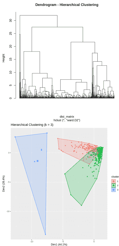
Hierarchical Clustering

3. DBScan Clustering

DBSCAN (Density-Based Spatial Clustering of Applications with Noise) is an unsupervised clustering algorithm that groups data points based on regions of high density. Unlike K-Means, it does not require the number of clusters to be specified in advance. DBSCAN can detect clusters of arbitrary shapes and effectively identify noise or outliers in the dataset.

• The algorithm selects a point and checks whether it has enough neighbouring points within a specified radius to form a dense region.
• If the minimum number of points is met, a cluster is formed and expanded by including all density-reachable points.
• Points that do not belong to any dense region are labeled as noise or outliers, making the method robust to irregular data distributions.

**Implementation: Here we implement DBSCAN clustering to the Iris dataset.

• The numeric features of the Iris dataset are selected and scaled to standardize the data before clustering.
• DBSCAN is applied using specified eps (neighborhood radius) and minPts (minimum points to form a cluster) parameters to detect dense regions and identify noise.
• The resulting clusters are visualized in 2D, where grouped points form clusters and isolated points are marked as outliers. R `

install.packages("dbscan") install.packages("factoextra")

library(dbscan) library(factoextra)

data <- iris[, 1:4]

scaled_data <- scale(data)

set.seed(123)

db <- dbscan(scaled_data, eps = 0.8, minPts = 5)

print(db)

fviz_cluster(db, data = scaled_data, geom = "point", main = "DBSCAN Clustering on Iris Dataset")

`

**Output:

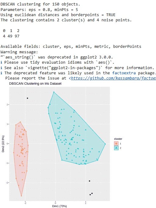
DBSCAN clustering

4. Fuzzy Clustering

Fuzzy Clustering also known as Fuzzy C-Means (FCM), is an unsupervised learning technique where each data point can belong to multiple clusters with different degrees of membership. Unlike hard clustering methods such as K-Means, which assign each point to only one cluster, fuzzy clustering provides a membership score between 0 and 1 for every cluster. This approach is especially useful when cluster boundaries are overlapping or not clearly defined.

• The algorithm initializes cluster centers and assigns each data point a membership value for every cluster based on distance.
• Cluster centers are updated using weighted averages, where weights are determined by membership scores.
• The process repeats until membership values stabilize and final clusters are formed based on the highest membership degree for each point.

**Implementation: Here we implement Fuzzy C-Means clustering to the mtcars dataset

• Installed and loaded the required libraries, selected the mtcars dataset and standardized the data using scale() to ensure fair distance calculations.
• The cmeans() function applies Fuzzy C-Means clustering with 3 centers, fuzziness parameter m = 2 and a maximum of 100 iterations.
• It produces membership values that indicate the degree to which each data point belongs to each cluster.
• Cluster assignments are extracted, converted into factors and visualized using fviz_cluster() with convex ellipses to display the clustered groups. R `

install.packages("e1071") install.packages("factoextra")

library(e1071) library(factoextra)

data <- mtcars scaled_data <- scale(data) set.seed(123)

fcm <- cmeans(scaled_data, centers = 3, m = 2, iter.max = 100)

print(fcm$membership)

clusters <- as.factor(fcm$cluster)

fviz_cluster(list(data = scaled_data, cluster = clusters), geom = "point", ellipse.type = "convex", main = "Fuzzy C-Means Clustering on mtcars Dataset")

`

**Output:

5. Spectral Clustering

Spectral Clustering is an advanced clustering technique that groups data points based on similarity by using concepts from graph theory and linear algebra. Instead of directly clustering the original data, it constructs a similarity graph and analyzes its structure using eigenvalues and eigenvectors. This approach is especially effective for detecting complex, non-convex and non-linearly separable clusters.

• Construct a similarity matrix and form a graph where data points are nodes and edges represent similarities.
• Compute the graph Laplacian matrix and extract its eigenvalues and eigenvectors to transform the data into a lower-dimensional spectral space.
• Apply a standard clustering algorithm on the transformed eigenvector space to obtain the final clusters.

**Implementation: Here we implement Spectral Clustering

• Spectral Clustering is applied using specc() to divide the data into three clusters.
• The cluster assignments are added to the original dataset as a new categorical variable for plotting.
• A scatter plot is created showing Sepal Length vs Sepal Width, with points colored by cluster, labeled by species and ellipses drawn to highlight cluster boundaries. R `

install.packages("kernlab") install.packages("ggplot2") install.packages("ggrepel")

library(kernlab) library(ggplot2) library(ggrepel)

data <- iris[, 1:4] scaled_data <- scale(data)

set.seed(123)

sc <- specc(scaled_data, centers = 3)

iris$Cluster <- as.factor(sc)

ggplot(iris, aes(x = Sepal.Length, y = Sepal.Width, color = Cluster)) +

geom_point(size = 3, alpha = 0.8) +

geom_text_repel(aes(label = Species), size = 3.5, box.padding = 0.4, point.padding = 0.3, max.overlaps = Inf) +

stat_ellipse(aes(group = Cluster), linetype = 2, linewidth = 0.8) +

labs(title = "Spectral Clustering of Iris Dataset", x = "Sepal Length", y = "Sepal Width", color = "Cluster") +

theme_minimal(base_size = 14) +

theme( plot.title = element_text(hjust = 0.5, face = "bold"), legend.position = "right" )

`

**Output:

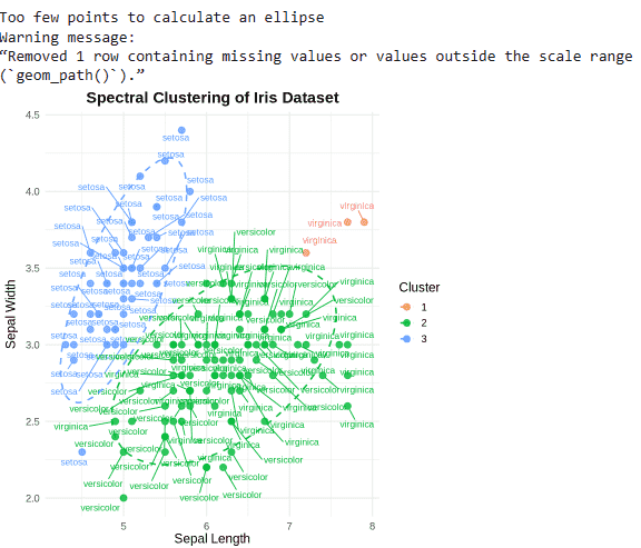
Spectral Clustering

**Ensemble Clustering

Ensemble Clustering is an advanced clustering approach that combines the results of multiple clustering algorithms or multiple runs of the same algorithm to produce a more stable and reliable final clustering solution. Instead of relying on a single method, it aggregates different clustering outcomes to reduce variability and improve robustness. This technique is especially useful when the true cluster structure is uncertain or when individual algorithms produce inconsistent results.

• Multiple clustering models (e.g., K-Means, Hierarchical, DBSCAN) are applied to the same dataset or the same algorithm is run multiple times with different parameters.
• The individual clustering results are combined using a consensus function, such as a co-association matrix or voting mechanism.
• A final clustering solution is generated from the aggregated results, improving stability and reducing the impact of noise or parameter sensitivity.

**Implementation

Here we implement Ensemble Clustering on the Wholesale Customers dataset.

• Three clustering methods (K-Means, Hierarchical and DBSCAN) are applied separately.
• The cluster outputs from all methods are combined into a matrix and majority voting is used to assign a final ensemble cluster to each observation.
• The final consensus clusters are added to the dataset and visualized to observe the overall grouping structure. R `

install.packages("dbscan") install.packages("kernlab") install.packages("factoextra")

library(dbscan) library(kernlab) library(factoextra)

data <- read.csv("Wholesale_Customers_Data.csv") numeric_data <- data[, c("Fresh", "Milk", "Grocery", "Frozen", "Detergents_Paper", "Delicassen")] scaled_data <- scale(numeric_data)

set.seed(123)

km <- kmeans(scaled_data, centers = 3, nstart = 25) cluster_km <- km$cluster

dist_matrix <- dist(scaled_data) hc <- hclust(dist_matrix, method = "ward.D2") cluster_hc <- cutree(hc, k = 3)

db <- dbscan(scaled_data, eps = 1.2, minPts = 5) cluster_db <- db$cluster

cluster_db[cluster_db == 0] <- max(cluster_db) + 1

clusters_matrix <- cbind(cluster_km, cluster_hc, cluster_db)

ensemble_cluster <- apply(clusters_matrix, 1, function(x) { as.numeric(names(sort(table(x), decreasing = TRUE)[1])) })

data$Ensemble_Cluster <- as.factor(ensemble_cluster)

fviz_cluster(list(data = scaled_data, cluster = ensemble_cluster), geom = "point", ellipse.type = "convex", main = "Ensemble Clustering - Wholesale Dataset")

`

**Output:

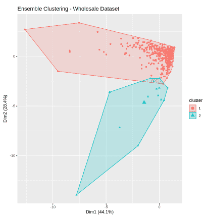
Ensemble Clustering

Download full code from here

Evaluation Metrics in Clustering

Clustering evaluation metrics help assess the quality and effectiveness of clustering results. These metrics measure how well data points are grouped within clusters and how distinct the clusters are from each other.

• Silhouette Score: Measures how similar a data point is to its own cluster compared to other clusters. Values range from -1 to 1, with higher values indicating better-defined and well-separated clusters.
• Davies–Bouldin Index (DBI): Evaluates clustering quality based on the ratio of within-cluster similarity to between-cluster separation. Lower values indicate more distinct and compact clusters.
• **Adjusted Rand Index (ARI): Compares predicted clusters with true labels and measures the level of agreement between them. Higher values indicate stronger similarity beyond random chance.
• **Within-Cluster Sum of Squares (WCSS): Measures the total variation within clusters by evaluating how close data points are to their centroids. Lower values represent tighter and more cohesive clusters.

Applications

• **Customer Segmentation: Clustering groups customers based on purchasing behavior and demographics, helping businesses create targeted marketing strategies and improve customer satisfaction.
• **Anomaly Detection: It identifies unusual data points that do not belong to any cluster, making it useful for fraud detection, fault diagnosis and cybersecurity monitoring.
• **Image Segmentation: Clustering divides images into regions with similar pixel characteristics, supporting object recognition and computer vision applications.
• **Medical Diagnostics: It groups patients with similar clinical features, assisting in disease classification and personalized treatment planning.
• **Financial Analysis: Clustering segments financial assets based on performance or risk patterns, helping in portfolio optimization and risk management.

Advantages

• Clustering does not require labeled data, making it suitable for exploratory data analysis.
• It helps discover hidden patterns and natural groupings within complex datasets.
• By grouping similar data points, it simplifies large datasets and improves interpretability.
• It is versatile and applicable across domains such as marketing, healthcare, finance and image analysis.

Limitations

• Many clustering algorithms require careful selection of parameters like the number of clusters or distance measures.
• Distance-based methods are sensitive to feature scaling and outliers.
• Interpreting clusters can be challenging and often requires domain expertise.
• Some algorithms are computationally expensive and may not scale well to very large datasets.