Decision Tree Classifiers in R Programming (original) (raw)

Last Updated : 18 Mar, 2026

Decision Tree is a machine learning algorithm that assigns new observations to predefined categories based on a training dataset. Its goals are to predict class labels for unseen data and identify the features that define each class. It has a flowchart-like tree structure in which the internal node represents feature(or attribute), the branch represents a decision rule and each leaf node represents the outcome.

A Decision Tree consists of

**Nodes: Test for the value of a certain attribute.
**Edges/Branch: Represents a decision rule and connect to the next node.
**Leaf nodes: Terminal nodes that represent class labels or class distribution.

**Example:

is_a_person_fit_

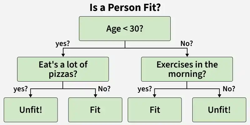
Decision Tree Structure

The diagram shows a decision tree that classifies a person as fit or unfit based on age, eating habits and exercise. If the person is under 30 and eats a lot of pizzas, they are unfit. If they do not eat a lot of pizzas, they are fit. If the person is 30 or older and exercises in the morning, they are fit. If they do not exercise, they are unfit.

Key characteristics of Decision Tree

Easy to interpret and visualize.
Capable of making automatic decisions.
Splits the feature space into smaller, manageable regions.

Implementation of Decision Tree Classifier in R

We will implement a decision tree classifier in R programming language to predict whether a person purchases a product based on their age and estimated salary, using the rpart package. The steps include data preprocessing, model training, evaluation and visualization.

**1. Installing and Loading Required Packages

We install and load the necessary libraries to build and visualize the decision tree.

**rpart: Used to train decision tree models.
**caTools: Helps in splitting the dataset into training and test sets.
**ggplot2: Used for creating visualizations.
**dplyr: Used for data manipulation and transformation. R `

install.packages("rpart") install.packages("caTools") install.packages("ggplot2") install.packages("dplyr")

library(rpart) library(caTools) library(ggplot2) library(dplyr)

**2. Loading the Dataset

We will use the Advertisement dataset which contains advertising expenditures across different media channels and their corresponding impact on product Sales. We will load the CSV file containing the dataset and preview the first few records. You can download the dataset from here.

**read.csv(): Loads a CSV file as a data frame.
**head(): Displays the first few rows of the dataset. R `

dataset <- read.csv("/content/Advertisement.csv") head(dataset, 10)

**Output:

dataset

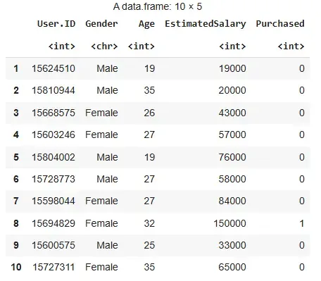
Output

**3. Preparing the Data

We encode the target variable as a factor and split the dataset into training and test sets.

**factor(): Converts a numeric variable into a categorical (factor) variable.
**sample.split(): Splits data into training and test parts randomly.
**subset(): Selects rows based on logical condition. R `

dataset$Purchased <- factor(dataset$Purchased, levels = c(0, 1))

set.seed(123) split <- sample.split(dataset$Purchased, SplitRatio = 0.75) training_set <- subset(dataset, split == TRUE) test_set <- subset(dataset, split == FALSE)

**4. Feature Scaling

We standardize the numerical features to ensure all values have the same scale.

**scale(): Normalizes numerical values to mean 0 and standard deviation 1. R `

training_set[c("Age", "EstimatedSalary")] <- scale(training_set[c("Age", "EstimatedSalary")]) test_set[c("Age", "EstimatedSalary")] <- scale(test_set[c("Age", "EstimatedSalary")])

**5. Fitting the Model

We train the decision tree classifier on the training data.

**rpart(): Builds a recursive partitioning tree.
**method = "class": Indicates that this is a classification problem. R `

classifier <- rpart(formula = Purchased ~ Age + EstimatedSalary, data = training_set, method = "class")

**6. Predicting the Test Set Results

We predict the class labels for the test data using the trained model.

**predict(): Predicts outcomes based on the model.
**type = "class": Ensures that the output is a class label, not a probability. R `

y_pred <- predict(classifier, newdata = test_set[c("Age", "EstimatedSalary")], type = "class")

**7. Evaluating the Model

We generate a confusion matrix and visualize it to understand the model’s performance.

**table(): Creates a confusion matrix.
**as.data.frame(): Converts matrix to a data frame for plotting.
**ggplot(): Used for creating advanced plots. R `

cm <- table(test_set$Purchased, y_pred)

cm_df <- as.data.frame(cm) colnames(cm_df) <- c("Actual", "Predicted", "Freq")

ggplot(cm_df, aes(x = Predicted, y = Actual)) + geom_tile(aes(fill = Freq), color = "white") + geom_text(aes(label = Freq), vjust = 0.5, fontface = "bold", size = 5) + scale_fill_gradient(low = "lightblue", high = "steelblue") + labs(title = "Confusion Matrix", x = "Predicted Label", y = "Actual Label") + theme_minimal()

**Output:

confusion_matrix

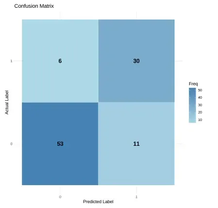
Output

**8. Visualizing Decision Boundaries (Training Set)

We create a grid of values and plot the decision boundary over the training data.

**expand.grid(): Creates a data frame from all combinations of input sequences.
**geom_point(), **scale_color_manual(): Used for plotting decision regions and class labels. R `

x_min <- min(training_set$Age) - 1 x_max <- max(training_set$Age) + 1 y_min <- min(training_set$EstimatedSalary) - 1 y_max <- max(training_set$EstimatedSalary) + 1

grid_set <- expand.grid( Age = seq(x_min, x_max, by = 0.01), EstimatedSalary = seq(y_min, y_max, by = 0.01) )

grid_set$Purchased <- predict(classifier, newdata = grid_set, type = "class")

ggplot() + geom_point(data = grid_set, aes(x = Age, y = EstimatedSalary, color = Purchased), alpha = 0.2) + geom_point(data = training_set, aes(x = Age, y = EstimatedSalary, shape = Purchased, fill = Purchased), size = 2) + labs(title = "Decision Tree Classification (Training Set)", x = "Age", y = "Estimated Salary") + scale_color_manual(values = c("tomato", "springgreen3")) + scale_fill_manual(values = c("red3", "green4")) + theme_minimal()

**Output:

training_plot

Output

**9. Visualizing Decision Boundaries (Test Set)

We repeat the visualization process for the test dataset to see how well the model generalizes.

R `

x_min <- min(test_set$Age) - 1 x_max <- max(test_set$Age) + 1 y_min <- min(test_set$EstimatedSalary) - 1 y_max <- max(test_set$EstimatedSalary) + 1

grid_set <- expand.grid( Age = seq(x_min, x_max, by = 0.01), EstimatedSalary = seq(y_min, y_max, by = 0.01) )

grid_set$Purchased <- predict(classifier, newdata = grid_set, type = "class")

ggplot() + geom_point(data = grid_set, aes(x = Age, y = EstimatedSalary, color = Purchased), alpha = 0.2) + geom_point(data = test_set, aes(x = Age, y = EstimatedSalary, shape = Purchased, fill = Purchased), size = 2) + labs(title = "Decision Tree Classification (Test Set)", x = "Age", y = "Estimated Salary") + scale_color_manual(values = c("tomato", "springgreen3")) + scale_fill_manual(values = c("red3", "green4")) + theme_minimal()

**Output:

test_plot

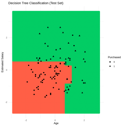
Output

**10. Plotting the Decision Tree Diagram

We plot the actual structure of the decision tree showing split criteria and class assignments.

**plot(): Draws the tree structure.
**text(): Labels the tree with split conditions and node values. R `

plot(classifier) text(classifier)

**Output:

decision_tree

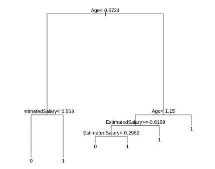
Output

The diagram shows a decision tree that classifies whether a person will purchase a product based on their age and estimated salary. It first checks if age is less than or equal to 44.5 and then further splits based on salary values. Each path ends in a prediction, either class 0 or 1, representing the model’s final decision.