Diabetes Prediction using R (original) (raw)
Last Updated : 23 Jul, 2025
In this article, we will learn how to predict whether a person has diabetes or not using the Diabetes dataset. This is a classification problem and we'll utilize Logistic Regression in R Programming Language to make our predictions.
**Project Overview
In this project, we aim to predict whether a person has diabetes based on their medical information. We will cover the following steps:
- **Loading the dataset: Import the necessary dataset and libraries.
- **Exploratory Data Analysis (EDA): Understand the dataset by visualizing distributions and correlations.
- **Preprocessing: Handle missing values, normalize features and split the dataset into training and testing sets.
- **Training the model: Build and train a **Logistic Regression model for diabetes prediction.
- **Evaluating the model: Use accuracy, precision, recall and other metrics to assess the model's performance.
- **Making predictions: Apply the model to predict the risk of diabetes for new data.
**Overview of dataset
The diabetes.csv dataset contains health metrics used to predict diabetes. Key features include:
- **Pregnancies: Number of times pregnant
- **Glucose: Plasma glucose concentration after a 2-hour oral test
- **BloodPressure: Diastolic blood pressure (mm Hg)
- **SkinThickness: Triceps skinfold thickness (mm)
- **Insulin: 2-hour serum insulin (mu U/ml)
- **BMI: Body Mass Index (kg/m²)
- **DiabetesPedigreeFunction: A score estimating genetic risk based on family history
- **Age: Age in years
- **Outcome: Target variable (0 = non-diabetic, 1 = diabetic)
Dataset Link: Diabetes Dataset
**1. Loading the Required Libraries and Dataset
We will begin by loading the necessary libraries and importing the dataset.
R `
library(readr) library(caTools) library(caret) library(e1071)
data <- read.csv("diabetes.csv") head(data)
`
**Output:
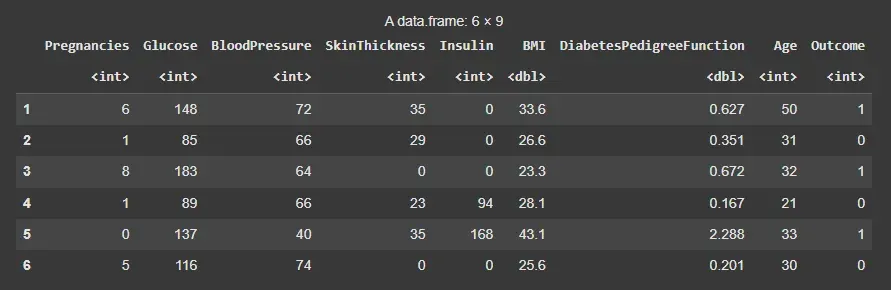
Dataset
This dataset contains eight features, each of which determines a result of 0 or 1. 0 means the patient does not have diabetes, whereas a score of 1 means they do.
**2. Data Preprocessing
In this step, we preprocess the data by handling missing values, scaling features and splitting the dataset:
- Checked for missing values using summary statistics.
- Separated features (X) and target variable (y).
- Scaled only the features to standardize their values (mean = 0, SD = 1).
- Recombined scaled features with the target to form the final dataset.
- Split data into training (70%) and testing (30%) sets using a fixed random seed for reproducibility. R `
summary(data)
colSums(is.na(data))
X <- data[, 1:8] y <- data[, 9]
scaled_X <- as.data.frame(scale(X))
scaled_data <- cbind(scaled_X, y)
X <- scaled_data[, 1:8] y <- scaled_data[, 9]
set.seed(123) sample <- sample.split(y, SplitRatio = 0.7) X_train <- X[sample == TRUE, ] y_train <- y[sample == TRUE] X_test <- X[sample == FALSE, ] y_test <- y[sample == FALSE]
`
**Output:
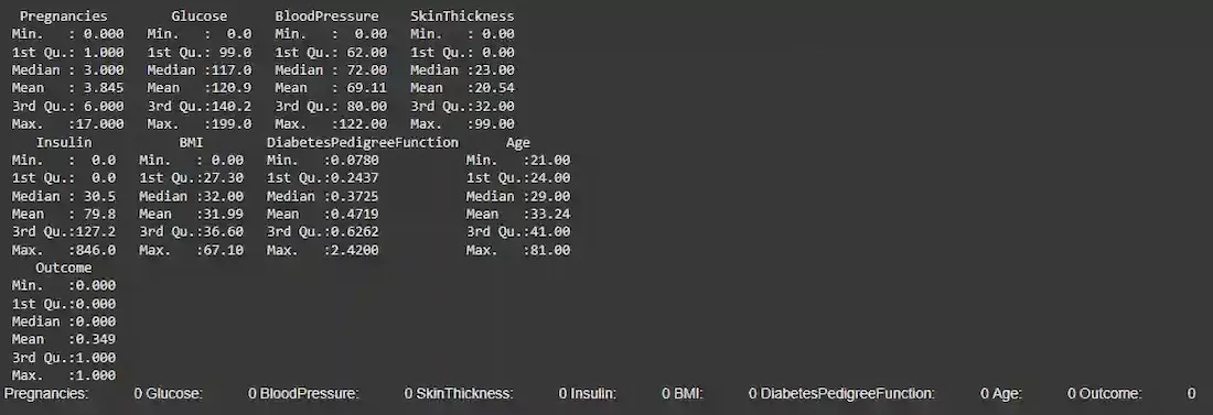
Data Preprocessing
We ensured that the dataset was clean by checking for missing values and scaling the columns. We then split the data into **training and **testing sets for later evaluation.
3. Exploratory Data Analysis (EDA)
Now we will create some visualization for this dataset to get explore our dataset.
3.1 Correlation Heatmap
We will visualize the correlations between various features using a **correlation heatmap. This will help us understand the relationships between different variables in the dataset.
R `
library(ggplot2) library(reshape2)
correlation_matrix <- cor(data)
correlation_melted <- melt(correlation_matrix)
ggplot(correlation_melted, aes(Var1, Var2, fill=value)) + geom_tile(color="white") + scale_fill_gradient2(low="blue", high="red", mid="white", midpoint=0, limit=c(-1,1), space="Lab", name="Correlation") + theme_minimal() + theme(axis.text.x = element_text(angle = 45, hjust = 1)) + labs(title="Correlation Heatmap", x="Features", y="Features")
`
**Output:
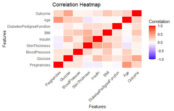
Predicting Diabetes Risk in R
The heatmap visualizes the **correlation matrix and provides insights into the strength and direction of relationships between the features.
3.2 Distribution of Diabetes Outcomes
Now, we will visualize the distribution of the **Outcome variable (whether or not a person has diabetes).
R `
outcome_counts <- table(data$Outcome) outcome_df <- data.frame(Outcome = names(outcome_counts), Count = as.numeric(outcome_counts))
ggplot(outcome_df, aes(x=Outcome, y=Count)) + geom_bar(stat="identity", fill="pink") + labs(title="Distribution of Diabetes Outcomes", x="Outcome", y="Count") + theme_minimal() + theme(axis.text.x = element_text(size=12), axis.text.y = element_text(size=12), axis.title = element_text(size=12), plot.title = element_text(size=16, face="bold"))
`
**Output:
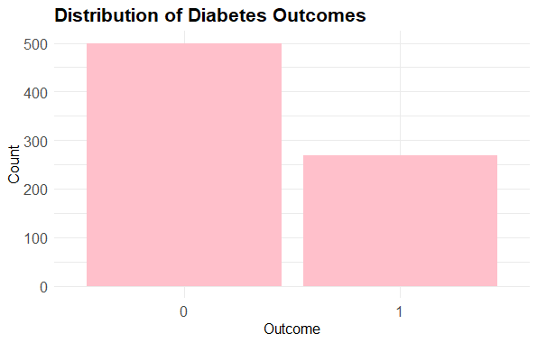
Predicting Diabetes Risk in R
This bar plot shows the distribution of **Outcome classes (0 for no diabetes and 1 for diabetes), helping us understand the balance between classes.
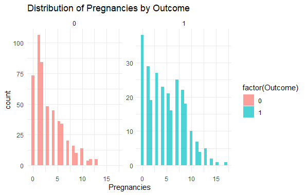
3.3 Histograms with Outcome Split
Next, we'll plot histograms for various features, split by the Outcome class, to understand how the distribution of each feature varies between diabetic and non-diabetic individuals.
R `
library(ggplot2)
diabetes_subset <- data[, c("Pregnancies", "Glucose", "BloodPressure", "BMI", "Age", "Outcome")]
ggplot(diabetes_subset, aes(x = Pregnancies, fill = factor(Outcome))) + geom_histogram(position = "identity", bins = 30, alpha = 0.7) + labs(title = "Distribution of Pregnancies by Outcome") + facet_wrap(~Outcome, scales = "free_y") + theme_minimal()
`
**Output:
Predicting Diabetes Risk in R
We visualized the distribution of **Pregnancies with respect to the **Outcome to identify patterns between the feature and the target variable.
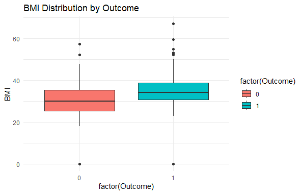
3.4 Boxplot for BMI by Outcome
To understand the distribution of **BMI for both diabetic and non-diabetic individuals, we can plot a **boxplot.
R `
library(ggplot2)
ggplot(data, aes(x = factor(Outcome), y = BMI, fill = factor(Outcome))) + geom_boxplot() + labs(title = "BMI Distribution by Outcome") + theme_minimal()
`
**Output:
Predicting Diabetes Risk in R
This boxplot shows how **BMI varies for individuals with and without diabetes. It helps to identify if there's a noticeable difference in BMI between the two classes.
**4. Building the Model
Now, we will build a **Logistic Regression model to predict diabetes based on medical features.
R `
log_model <- glm(y_train ~ ., data = X_train, family = binomial)
summary(log_model)
`
**Output:
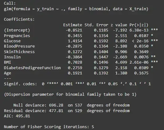
Model Building
**5. Evaluating the Model
To evaluate the model, we will calculate various performance metrics like **accuracy, **precision, **recall and **F1 score using the test data.
R `
predictions <- predict(log_model, newdata = X_test, type = "response")
predictions <- factor(ifelse(predictions > 0.5, 1, 0), levels = levels(as.factor(y_test)))
confusionMatrix(predictions, as.factor(y_test))
`
**Output:
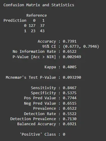
Evaluating the Model
**6. Making Predictions using the Model
We will now use the trained model to predict the likelihood of diabetes for a new patient based on their medical data. This function allows us to predict diabetes risk for a new patient by entering their medical parameters. The prediction is based on the trained logistic regression model.
R `
predict_diabetes <- function(pregnancies, glucose, bloodpressure, skinthickness, insulin, bmi, diabetespedigreefunction, age) { input_data <- data.frame( Pregnancies = pregnancies, Glucose = glucose, BloodPressure = bloodpressure, SkinThickness = skinthickness, Insulin = insulin, BMI = bmi, DiabetesPedigreeFunction = diabetespedigreefunction, Age = age ) input <- as.data.frame(input_data) prediction <- predict(log_model, newdata = input, type = "response") prediction <- factor(ifelse(prediction > 0.5, 1, 0), levels = levels(as.factor(prediction)))
return(prediction) }
new_patient <- data.frame( pregnancies = 6, glucose = 148, bloodpressure = 72, skinthickness = 35, insulin = 0, bmi = 33.6, diabetespedigreefunction = 0.627, age = 50 )
prediction <- predict_diabetes( new_patient$pregnancies, new_patient$glucose, new_patient$bloodpressure, new_patient$skinthickness, new_patient$insulin, new_patient$bmi, new_patient$diabetespedigreefunction, new_patient$age )
if (any(prediction == 1)) { cat("Based on the model's prediction, there is a higher chance of diabetes.") } else { cat("Based on the model's prediction, the risk of diabetes appears lower.") }
`
**Output:
Based on the model's prediction, there is a higher chance of diabetes.
Conclusion
From our analysis, we:
- Explored the distribution of diabetes outcomes and analyzed key variables such as Glucose and BMI.
- Conducted exploratory data analysis (EDA) to uncover relationships between features.
- Built a Logistic Regression model for diabetes prediction with relatively good accuracy, but with room for improvement in recall.
We concluded that the logistic regression model is effective for predicting diabetes. However, further model optimization and data balancing techniques could improve the recall, making the model more robust in identifying diabetic patients.