How to Use lm() Function in R to Fit Linear Models? (original) (raw)
Last Updated : 23 Jul, 2025
In this article, we will learn how to use the lm() function to fit linear models in the R Programming Language.
A linear model is used to predict the value of an unknown variable based on independent variables. It is mostly used for finding out the relationship between variables and forecasting. The lm() function is used to fit linear models to data frames in the R Language. It can be used to carry out regression, single stratum analysis of variance, and analysis of covariance to predict the value corresponding to data that is not in the data frame. These are very helpful in predicting the price of real estate, weather forecasting, etc.
To fit a linear model in the R Language by using the lm() function, We first use data.frame() function to create a sample data frame that contains values that have to be fitted on a linear model using regression function. Then we use the lm() function to fit a certain function to a given data frame.
Syntax:
lm( fitting_formula, dataframe )
Parameter:
- fitting_formula: determines the formula for the linear model.
- dataframe: determines the name of the data frame that contains the data.
Then, we can use the summary() function to view the summary of the linear model. The summary() function interprets the most important statistical values for the analysis of the linear model.
Syntax:
summary( linear_model )
The summary contains the following key information:
- Residual Standard Error: determines the standard deviation of the error where the square root of variance subtracts n minus 1 + # of variables involved instead of dividing by n-1.
- Multiple R-Squared: determines how well your model fits the data.
- Adjusted R-Squared: normalizes Multiple R-Squared by taking into account how many samples you have and how many variables you’re using.
- F-Statistic: is a “global” test that checks if at least one of your coefficients is non-zero.
Example: Example to show usage of lm() function.
R `
sample data frame
df <- data.frame( x= c(1,2,3,4,5), y= c(1,5,8,15,26))
fit linear model
linear_model <- lm(y ~ x^2, data=df)
view summary of linear model
summary(linear_model)
`
Output:
Call:
lm(formula = y ~ x^2, data = df)
Residuals:
1 2 3 4 5
2.000e+00 5.329e-15 -3.000e+00 -2.000e+00 3.000e+00
Coefficients:
Estimate Std. Error t value Pr(>|t|)
(Intercept) -7.0000 3.0876 -2.267 0.10821
x 6.0000 0.9309 6.445 0.00757 **
---
Signif. codes: 0 ‘***’ 0.001 ‘**’ 0.01 ‘*’ 0.05 ‘.’ 0.1 ‘ ’ 1
Residual standard error: 2.944 on 3 degrees of freedom
Multiple R-squared: 0.9326, Adjusted R-squared: 0.9102
F-statistic: 41.54 on 1 and 3 DF, p-value: 0.007575
Diagnostic Plots
The diagnostic plots help us to view the relationship between different statistical values of the model. It helps us in analyzing the extent of outliers and the efficiency of the fitted model. To view diagnostic plots of a linear model, we use the plot() function in the R Language.
Syntax:
plot( linear_model )
Example: Diagnostic plots for the above fitted linear model.
R `
sample data frame
df <- data.frame( x= c(1,2,3,4,5), y= c(1,5,8,15,26))
fit linear model
linear_model <- lm(y ~ x^2, data=df)
view diagnostic plot
plot(linear_model)
`
Output:

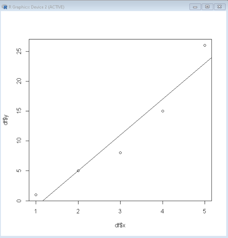
Plotting Linear model
We can plot the above fitted linear model to visualize it well by using the abline() method. We first plot a scatter plot of data points and then overlay it with an abline plot of the linear model by using the abline() function.
Syntax:
plot( df$x, df$y)
abline( Linear_model )
Example: Plotting linear model
R `
sample data frame
df <- data.frame( x= c(1,2,3,4,5), y= c(1,5,8,15,26))
fit linear model
linear_model <- lm(y ~ x^2, data=df)
Plot abline plot
plot( df$x, df$y ) abline( linear_model)
`
Output:
Predict values for unknown data points using the fitted model
To predict values for novel inputs using the above fitted linear model, we use predict() function. The predict() function takes the model and data frame with unknown data points and predicts the value for each data point according to the fitted model.
Syntax:
predict( model, data )
Parameter:
- model: determines the linear model.
- data: determines the data frame with unknown data points.
Example: Predicting novel inputs
R `
sample data frame
df <- data.frame( x= c(1,2,3,4,5), y= c(1,5,8,15,26))
fit linear model
linear_model <- lm(y ~ x^2, data=df)
Predict values
predict( linear_model, newdata = data.frame(x=c(15,16,17)) )
`
Output:
1 2 3
83 89 95