Implement Machine Learning With Caret In R (original) (raw)

Last Updated : 23 Jul, 2025

Machine Learning (ML) is a method where computers learn patterns from data and make predictions or decisions without being explicitly programmed. It’s widely used in real-world applications like spam filtering, medical diagnosis, stock prediction and image recognition.

**Example: A hospital uses machine learning to predict if a patient has diabetes by analyzing their age, blood sugar levels, BMI and other medical information. This helps doctors make quicker and more accurate diagnoses.

What is Caret in R?

Caret stands for Classification And Regression Training. It is an R package that helps us build ML models. With Caret, we can:

Clean and prepare data
Split data into training and test sets
Train different ML models
Test model accuracy

Caret supports many algorithms like decision trees, SVM and LDA. We can use the same simple train() function for all.

Implementing Machine Learning with Caret in R

We will now implement a LDA model in R programming language using the caret library

1. Installing required packages

We install the necessary libraries used for data handling, visualization and modeling.

**install.packages(): Installs external packages from CRAN so we can use their functions.
**ggplot2: Used to create data visualizations like bar plots, histograms and boxplots.
**ggpubr: Enhances ggplot2 by making it easier to create clean, publication-ready plots.
**reshape: Helps reshape and organize data, especially useful for converting data into long format with melt().
**caret: Main package for building machine learning models, including training, testing and evaluation.
**kernlab: Provides backend support for models like SVM that are used by caret. R `

install.packages("ggplot2") install.packages("ggpubr") install.packages("reshape") install.packages("caret") install.packages("kernlab")

2. Loading installed libraries

We load all required libraries into our current R session.

**library(): Activates packages like ggplot2, caret, etc., for use in the script. R `

library(ggplot2) library(ggpubr) library(reshape) library(caret) library(kernlab)

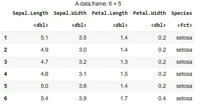
3. Importing and Viewing the Dataset

We import the built-in iris dataset and check the top rows to understand its structure.

**data(): Loads the iris dataset into memory.
**head(): Displays the first few rows of the dataset. R `

data("iris") head(iris)

**Output:

head_data

Output

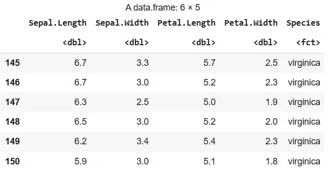
4. Viewing the Last Few Rows

We view the bottom rows of the dataset to complete our inspection.

**tail(): Displays the last few rows. R `

tail(iris)

**Output:

tail_data

Output

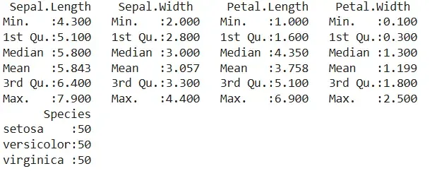
5. Generating Summary Statistics

We summarize the dataset to understand distributions and detect anomalies.

**summary(): Provides a statistical summary of each column. R `

summary(iris)

**Output:

summary_data

Output

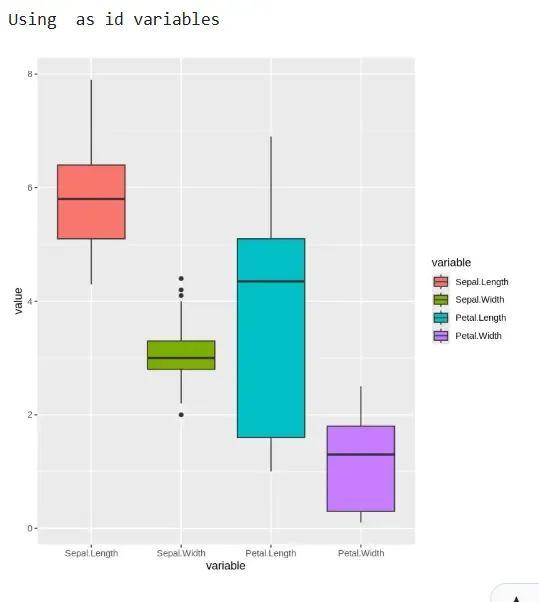
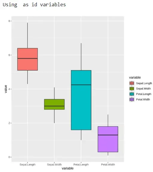
6. Detecting Outliers with Boxplots

We identify potential outliers among numeric variables.

**subset(): Selects only numeric columns.
**melt(): Reshapes data for plotting.
**ggplot() + geom_boxplot(): Creates boxplots for each variable. R `

df <- subset(iris, select = c(Sepal.Length, Sepal.Width, Petal.Length, Petal.Width)) ggplot(data = melt(df), aes(x = variable, y = value)) + geom_boxplot(aes(fill = variable))

**Output:

boxplot

Output

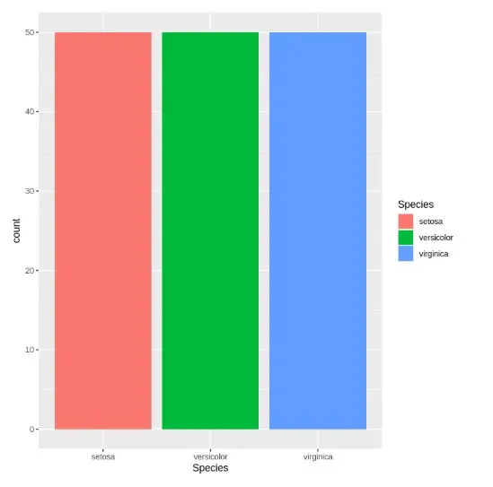
7. Plotting Categorical Variable Distribution

We visualize how different categories are distributed.

**ggplot() + geom_bar(): Creates bar plots for the Species column. R `

ggplot(data = iris, aes(x = Species, fill = Species)) + geom_bar()

**Output:

plot

Output

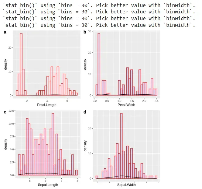
8. Visualizing Histograms of Numeric Variables

We visualize the distribution of numeric variables using histograms and density.

**ggplot() + geom_histogram() + geom_density(): Plots histograms overlaid with density curves.
**ggarrange(): Arranges multiple plots. R `

a <- ggplot(data = iris, aes(x = Petal.Length)) + geom_histogram(color = "red", fill = "blue", alpha = 0.01) + geom_density() b <- ggplot(data = iris, aes(x = Petal.Width)) + geom_histogram(color = "red", fill = "blue", alpha = 0.1) + geom_density() c <- ggplot(data = iris, aes(x = Sepal.Length)) + geom_histogram(color = "red", fill = "blue", alpha = 0.1) + geom_density() d <- ggplot(data = iris, aes(x = Sepal.Width)) + geom_histogram(color = "red", fill = "blue", alpha = 0.1) + geom_density() ggarrange(a, b, c, d + rremove("x.text"), labels = c("a", "b", "c", "d"), ncol = 2, nrow = 2)

**Output:

gplot

Output

9. Splitting the Dataset

We split the dataset into training and testing sets.

**createDataPartition(): Creates training and testing partitions. R `

limits <- createDataPartition(iris$Species, p = 0.80, list = FALSE) testiris <- iris[-limits, ] trainiris <- iris[limits, ]

10. Identifying and Removing Outliers

We clean the training data by removing outliers based on IQR.

**quantile(): Calculates 25th and 75th percentiles.
**IQR(): Computes interquartile range.
**subset(): Filters rows within bounds. R `

Q <- quantile(trainiris$Sepal.Width, probs = c(.25, .75), na.rm = FALSE) iqr <- IQR(trainiris$Sepal.Width) up <- Q[2] + 1.5 * iqr low <- Q[1] - 1.5 * iqr normal <- subset(trainiris, trainiris$Sepal.Width > low & trainiris$Sepal.Width < up)

11. Rechecking Data After Outlier Removal

We visualize the cleaned data to confirm removal of outliers.

**subset(): Selects numeric columns again.
**melt(): Reshapes cleaned data.
**ggplot() + geom_boxplot(): Plots boxplots post-cleaning. R `

boxes <- subset(normal, select = c(Sepal.Length, Sepal.Width, Petal.Length, Petal.Width)) ggplot(data = melt(boxes), aes(x = variable, y = value)) + geom_boxplot(aes(fill = variable))

**Output:

box_plot

Output

12. Setting Up Cross-Validation Parameters

We configure model evaluation using 10-fold cross-validation.

**trainControl(): Sets validation strategy.
**metric: Defines accuracy as evaluation metric. R `

crossfold <- trainControl(method = "cv", number = 10, savePredictions = TRUE) metric <- "Accuracy"

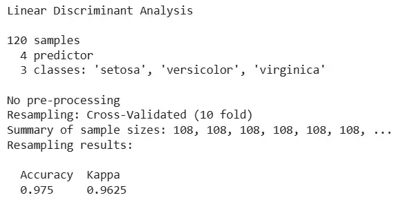
13. Training the LDA Model

We train the LDA model using the training set.

**train(): Fits LDA using defined metric and cross-validation. R `

set.seed(42) fit.lda <- train(Species ~ ., data = trainiris, method = "lda", metric = metric, trControl = crossfold)

**Output:

Linear_discriminant

Output

14. Making Predictions and Evaluating Accuracy

We evaluate the LDA model’s performance on test data.

**predict(): Generates predictions on test data.
**confusionMatrix(): Compares predicted vs actual values. R `

predictions <- predict(fit.lda, testiris) confusionMatrix(predictions, testiris$Species)

**Output:

confusion_matrx_and_plot

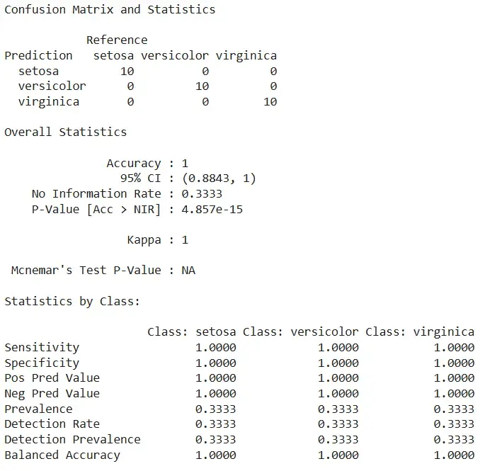
Output

The model achieved perfect classification with 100% accuracy, correctly predicting all species in the test set without any errors.